Software-Integrated FLIM for Nikon A1+ Confocals
Abstract: FLIM operation with the bh TCSPC/FLIM
modules has been implemented in the new NIS-Elements software of the Nikon A1+
confocal laser confocal laser scanning microscopes. The systems use one or two
bh BDS-SM picosecond diode lasers, two bh HPM-100 hybrid detectors, and two
fully parallel SPC-150N TCSPC data recording channels. All FLIM components are
controlled via Nikons NIS-Elements software. Intensity images, FLIM images,
and decay curves from regions of interest are displayed online. For precision
multi-exponential data analysis, the system incorporates bhs SPCImage FLIM
data analysis software.
Principle of Signal Recording
The sample is scanned with the focused beam
of a high-frequency pulsed laser. The laser excites fluorescence in the sample.
The fluorescence signal is collected by the microscope lens, fed back through
the beam path of the scanner, separated from the excitation light, sent through
a confocal pinhole, and, finally, detected by an optical detector. Compared
with wide-field imaging by a camera the scanning process has several advantages.
The first one is that the pinhole passes light only from the focal plane of the
microscope lens. The images are thus free of the typical out-of focus-haze seen
in normal visual microscopes. Moreover, there is no problem with scattering. A
wide-field system, in every pixel, records scattered light from all other
pixels and focal planes. A scanning system does not have this problem. It
excites only one pixel at a time, and detects only from this pixel and within a
well-defined sample plane. Thus, confocal scanning delivers clean images from a
selected plane in the sample which are free of lateral and longitudinal
crosstalk.
The detection system is based on bhs
multi-dimensional TCSPC process. The light passing the pinhole is sent to a
single-photon sensitive detector. The TCSPC system receives the photon pulses
from the detector together with the pixel, line, and frame clock pulses from
the scanner. For every photon, it determines the time of the photon after the
laser pulse and the position of the laser beam in the sample in the moment when
the photon was detected. The result is a photon distribution over the detection
time and the scan coordinates. The distribution can be considered an array of
pixel, each of which containing a fluorescence decay curve in the form of
photon numbers in consecutive time channels [1, 2, 3, 4].
TCSPC FLIM has a number of other intriguing
features. The most important ones are the time resolution and the sensitivity.
The time resolution of the TCSPC process is only limited by the laser pulse
width and the transit-time jitter in the detector. The resulting
instrument-response function (IRF) is 10 to 20 times narrower than for a
system that uses the same detector in combination with an analog-recording
system [1, 5]. At the same
time, the system delivers near-ideal sensitivity. Every photon seen by the
detector is ending up in the result. For a given number of photons, N, in a
particular pixel the signal-to-noise ratio for the obtained fluorescence lifetime
is close to N1/2, the ideal value for any optical measurement [1, 2].
There is a number of other advantages of
TCSPC FLIM, such as the capability to record multi-wavelength FLIM [6], to quasi-simultaneously
record a several excitation wavelengths [1, 2], to record extremely fast
time-series [1, 9], or simultaneously record FLIM and PLIM [7, 8]. These
features of the bh FLIM technique are not (yet) implemented in Nikons NIS-Elements
software. However, they can be used by running bh SPCM data acquisition
software in parallel with Nikon Elements microscope software.
Architecture
The basic system uses a bh BDS-SM picosecond
diode laser [10] for excitation, two bh HPM-100-40 hybrid detectors [1] for detecting the photons, and two
parallel bh SPC-150N TCSPC / FLIM modules for recording the data [1]. The laser
and the detectors are controlled by one DCC-100 Detector/Laser controller
module each. The SPC and DCC modules are operated in an extension box connected
to the NIKON system computer. The general system architecture is shown in Fig. 1.
Fig. 1:
Architecture of the NINKON integrated FLIM system
Two modifications of the system are
possible without changes in the Nikon integrated FLIM software:
- Additional lasers can be added to the system. The output beams of
up to four lasers can be combined into a single optical fibre and delivered
into the scan head.
- One detector or both detectors can be replaced with ultra-fast
HPM-100-06 detectors [5]. With these detectors, the instrument-response
function (IRF) is essentially determined by the laser. With 375nm, 405 nm,
and 445 nm lasers, the IRF width is about 40 ps. For lasers of 473,
488, and 515 nm the FWHM is between 60 ps and 90 ps.
Other extensions, like a multi-wavelength
detector [1], bh FASTAC FLIM [12],
or simultaneous FLIM/PLIM [7] can
be added and operated via bh SPCM software running in parallel with Nikons NIS-Elements
software.
Software
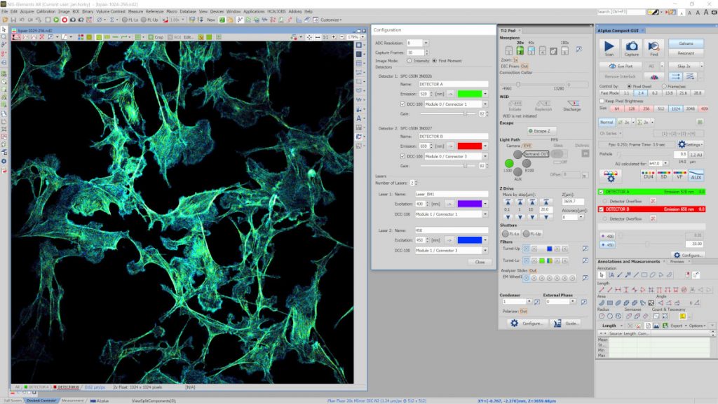
A typical panel configuration of the FLIM
implementation in Nikons NIS-Elements software is shown in Fig. 2. The FLIM
system has two TCSPC channels and two lasers. A lifetime image is shown for one
of the FLIM channels is shown on the left. The control panels for the FLIM
acquisition and the scan parameters are shown on the right. The panel next
right to the FLIM image controls the FLIM acquisition. With the setting shown, 30
Frames are accumulated. One channel records through a 520 nm filter, the
other through a 650 nm filter. Lifetime images are calculated online by a
first-moment algorithm [11]. The microscope parameters and spatial imaging
parameters are defined via the two panels on the right. Image size is
1024 x 1024 pixels, the acquisition is started by clicking on Capture
(right panel).
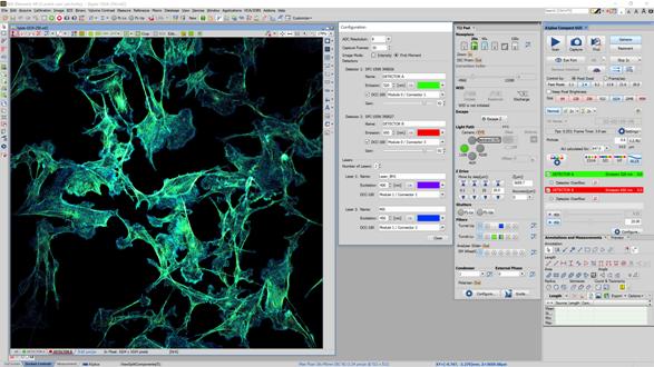
Fig. 2: Implementation of FLIM in Nikon NIS-Elements. Control panels: FLIM
configuration, light path configuration, and scan parameter definitions.
Simultaneous display of the lifetime images
of both FLIM channels is shown in Fig. 3. The FLIM configuration and the Ti2
Microscope control panel were closed to provide space for the second image.
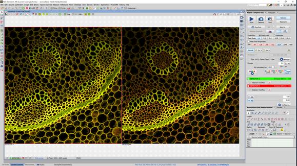
Fig. 3: Convallaria sample, scanned with 1024 x 1024 pixels,
Lifetime by First-Moment analysis, images of both FLIM channels displayed.
Online FLIM display can be combined with
displaying decay curves from the entire images or from regions of interest. An
example is shown in Fig. 4.

Fig. 4:
Display of decay functions from the entire images or from regions of interest.
FLIM with the 'Large-Image' function of the
Nikon system is shown in Fig. 5. The principle is equivalent to the Mosaic
FLIM capability of the bh SPCM software [1]: A part of the sample is scanned,
then the sample is offset by the scan-field diameter, and the sample is scanned
again. the process is continued until the desired are of the sample has been
imaged. The corresponding scans are combined into a single, large image. The
advantage is that a large sample are can be covered by a high-NA microscope
lens, delivering high lateral and longitudinal resolution, and high
light-collection efficiency.
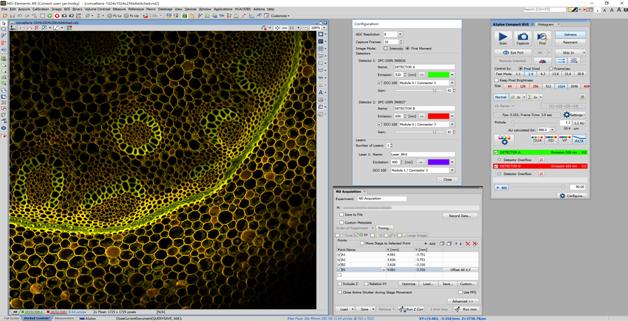
Fig. 5: Mosaic of four 1024x1024-pixel FLIM recordings, stitched together
giving a single 2048x2048 pixel image.
Multi-Exponential Data Analysis with bh SPCImage
Online lifetime calculation in NIS-Elements
delivers the lifetime for a single-exponential approximation of the decay data
in the pixels. For detailed analysis, bh SPCImage [1] has been embedded in the NIKON Elements
FLIM software. FLIM data are sent to SPCImage by a right mouse click and
selecting Send to SPCImage.
An example is shown in Fig. 6. The data are
the same as shown in Fig. 3, left image. The example shows an
amplitude-weighted lifetime image obtained from the components of a
double-exponential fit.
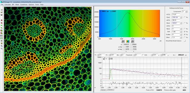
Fig. 6: SPCImage Data Analysis. Main panel, with lifetime image, lifetime
histogram, and decay curve at cursor position.
SPCImage is able to show also images of the
component lifetimes, t1 and t2, and of the amplitude ratio, a1/a2. Images for
these parameters are shown in Fig. 7. Biologically, these parameters are often
more meaningful than the amplitude-weighted or intensity-weighted lifetime.
Depending on the systems investigated, ratio images of bound and unbound NADH,
FRET efficiencies, and the ratio of interacting and non-interacting FRET Donor
can be derived. A phasor plot is available as well (Fig. 7 lower right),
providing extended options of image segmentation and decay analysis of combined
pixels. Please see [1] or [13] for details.
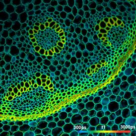
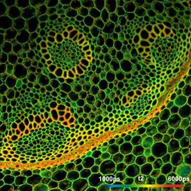
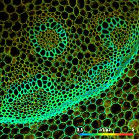

Fig. 7, upper left to lower right: Lifetime image of fast decay component,
t1, lifetime image of slow decay component, t2, colour-coded image of amplitude
ratio of the components, a1/a2, and phasor plot. All images 1024 x 1024 pixels.
Summary
The bh / Nikon A1 integrated FLIM system
provides an easy way to record FLIM data by a laser scanning microscope. Nikon NIS-Elements
mainly provides entry-level FLIM functions, and thus does not require special
knowledge about TCSPC and data recording procedures. Nevertheless, the system
records data with high photon efficiency, high signal-to-noise ratio, and high
time resolution. High-level multi-dimensional recording functions are available
by simply running bh SPCM data acquisition software in parallel with Nikon
Elements.
References
1.
W. Becker, The bh TCSPC handbook. 8th edition. Becker
& Hickl GmbH (2019), available on www.becker-hickl.com, please contact bh for printed
copies.
2. W. Becker (ed.), Advanced time-correlated single photon counting
applications. Springer, Berlin, Heidelberg, New York (2015)
3. W. Becker, Advanced time-correlated single-photon counting techniques. Springer, Berlin, Heidelberg, New York, 2005
4. W. Becker, Fluorescence Lifetime Imaging - Techniques and
Applications. J. Microsc. 247 (2) (2012)
5. Becker & Hickl GmbH, Sub-20ps IRF Width from Hybrid Detectors
and MCP-PMTs. Application note, available on www.becker-hickl.com
6.
W. Becker, A. Bergmann, C. Biskup, Multi-Spectral
Fluorescence Lifetime Imaging by TCSPC. Micr. Res. Tech. 70, 403-409 (2007)
7. Becker & Hickl GmbH, Simultaneous Phosphorescence and
Fluorescence Lifetime Imaging by Multi-Dimensional TCSPC and Multi-Pulse
Excitation. Application note, www.becker-hickl.com
8. W. Becker, V. Shcheslavskiy, A. Rück, Simultaneous phosphorescence
and fluorescence lifetime imaging by multi-dimensional TCSPC and multi-pulse excitation.
In: R. I. Dmitriev (ed.), Multi-parameteric live cell microscopy of 3D tissue
models. Springer (2017)
9. W. Becker, S. Frere, I. Slutsky, Recording Ca++ Transients in Neurons by TCSPC
FLIM. In:F.-J. Kao, G. Keiser, A. Gogoi, (eds.), Advanced optical methods of
brain imaging. Springer (2019)
10. BDS-SM Family picosecond diode lasers. Extended data sheet,
www.becker-hickl.com
11. Becker & Hickl GmbH, SPCM Software Runs Online-FLIM at 10 Images
per Second. Application note, available on www.becker-hickl.com
12. Becker & Hickl GmbH, Fast-Acquisition TCSPC FLIM System with
sub-25 ps IRF Width. Application note, available on www.becker-hickl.com
13. New SPCImage Version Combines Time-Domain Analysis with Phasor Plot.
Application note, www.becker-hickl.com
Contact:
Becker & Hickl GmbH
Nunsdorfer Ring 7-9
12277 Berlin, Germany
Tel. +49 30 212 800 20, Fax. +49 30 212 800 213
email: info@becker-hickl.com, https://www.becker-hickl.com