Wide-Field TCSPC FLIM with bh SPC-150 N TCSPC System and Photek FGN 392-1000 Detector
Wolfgang Becker, Holger
Netz, Becker & Hick GmbH, Berlin, Germany
Klaus Suhling, King's College London
Abstract:
We present a wide-field TCSPC FLIM system consisting of a position-sensitive
MCP PMT of the delay-line type, three SPC-150N TCSPC modules, a bh BDS-SM
picosecond diode laser, an inverted microscope, and optics that projects a
fluorescence image on the active area of the detector. The operation of the
system is fully integrated in the bh SPCM TCSPC software, data analysis is
performed by bh SPCImage. The system is able to record FLIM data with 1024 time
channels and up to 1024 x 1024 pixels. The effective spatial resolution
of the detector / TCSPC combination is about 250 x 250 pixels fwhm,
corresponding to about 160 µm on the active area of the detector.
Detector Principle
Wide-field imaging by photon counting is
around for more than a decade. Wide-field TCSPC techniques are based an
single-photon detection, generation of a position signal for each photon, and
building up the distribution of the photon number over the image coordinates.
In case of FLIM also the time of the individual detection events is determined,
and added as a coordinate of the photon distribution. The position information
can be derived form the electric charge of the individual photon pulses at the
outputs of a quadrant anode, a wedge-and-strip anode, or a resistive anode [1].
These principles require charge detection by low-noise noise charge-sensitive
amplifiers, analog-to digital conversion, and calculation of quotients of the
signals. These are time-consuming operations. The maximum count rate of such
systems is therefore low. Another way to obtain position information is to couple
the single-photon pulses into two crossed delay lines at the detector output.
The position is then determined by measuring the arrival times of the photon
pulses at the four outputs of the delay lines [1]. The delay lines can be
placed inside the detector, or outside the detector and coupled capacitively to
an inside resistive anode. The delay-line technique requires relatively complex
recording electronics but works up to a count rate of about 1 MHz. The principle
is shown in Fig. 1.
Fig. 1: Principle of position-sensitive detector: The detector has a
delay-line structure as an anode. The X position of a photon is proportional to
the delay between X1 and X2. The Y position of a photon is proportional to the
delay between Y1 and Y2. The time of the photon is derived from a signal from
the low-side of the channel plate, t.
TCSPC System
The TCSPC system consists of three parallel
SPC‑150N modules, see Fig. 2. The first module measures the times of the
photons in the laser pulse period. The second and third module measure the
times of the pulses at the outputs of the X and the Y delay lines. Delay cables
in the stop lines guarantee that the start-stop times remain positive for all X
and Y positions. The SPC modules are working in the FIFO (Parameter-TAG) mode [2].
That means the detection events, i.e. the times, t, and the positions, x and y,
are transferred into the computer photon by photon together with a macro
time. The macro time is an absolute time from the start of the acquisition. It
is used by the software to assign the t, x, and y data delivered by different
modules to a particular photon. From these data the software builds up a photon
distribution over the coordinates x, y, and the times, t. This is the usual
photon distribution of FLIM: It is an array of pixels, each of which contains a
fluorescence decay curve consisting of photon numbers in consecutive time
channels. To make this process possible the measurement in all three modules
must be started at exactly the same moment, and the macro-time clocks in the
modules must be synchronised. This is achieved by the Trigger Master and
Clock Master functions of the SPC-150N modules [2].
Fig. 2: TCSPC
System
Constant-Fraction Discriminators
All bh SPC modules have constant fraction
discriminators (CFDs) at their start and stop inputs. The CFDs not only reject
noise and low-amplitude pulses but also prevent the amplitude jitter of the
detector pulses from inducing timing jitter. For this purpose, the CFD circuitry
shapes the detector pulses into a bipolar waveform. The zero-cross point of
this pulse does not shift with the amplitude. A fast discriminator triggers on
the zero-cross point and thus delivers the temporal position of the photon is
independently of the pulse amplitude [1, 2]. If the pulse shaping network is
adapted to the rise and fall time of the detector pulses this principle works
well for all commonly used detectors. It also works for the single photon
pulses at the timing output of the Photek FGN 392-1000 detector, see Fig.
3, left. A normal CFD does not work, however, for the signals delivered by the
position outputs of a delay-line detector. The signals at these outputs have
nothing in common with normal single-photon pulses, see Fig. 3, middle. They resemble
of a burst of pulses rather than a single photon pulse. Trying to process a
signal like this by a normal CFD is hopeless.
The reason of the strange signal shape is
that the electron cloud of a single photoelectron simultaneously hits several
parts of the delay line structure, see Fig. 1. Moreover, the subsequent steps
of the delay line are electrically not perfectly de-coupled. The only way to
obtain timing from the position outputs is to determine the centroid of the
entire burst. This can be achieved by sending the signal through a low-pass
filter (pulse shape shown in Fig. 3, right) and processing the resulting pulse
by a CFD that has an appropriately designed pulse shaping network [3]. The
unavoidable side effect is that the filtered signal is slow, and that accurate
timing on it becomes difficult. This sets a limit to the spatial resolution of
the detector / TCSPC combination.
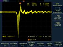
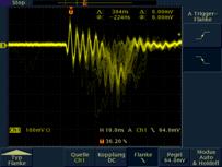

Fig. 3: Single photon pulses delivered by the Photek detector. Left:
Timing output. Middle: Position output X1. Right: Signal of position output X1
after passing through a 20 MHz low-pass filter.
The SPC-150N modules in the two position
channels have special CFDs (WF type). The WF CFDs have a pulse shaping
network which simultaneously acts as a low-pass filter. The result is smooth
timing on the position signals, and interpolation of the effective time of the
signal over the discrete steps of the delay line structure [3].
Optical System
The optical part of the wide-field FLIM
system is shown in Fig. 4. It consists of an inverted microscope, a BDS-SM
488nm picosecond diode laser, and a Photek FGN 392-1000 detector. The BDS-SM
laser is used for excitation. A cleaning filter removes long-wavelength
broadband emission from the laser beam. The light passing the filter is
delivered into the microscope by a single-mode fibre. A standard microscope
beam-splitter cube reflects the laser towards the microscope lens. The fibre output
delivers a diverging beam of light into the back aperture of the microscope
lens. The light is thus not focused into the sample, it illuminates the entire
field of view. Due to the clean beam profile at the end of the single-mode fibre
the illumination is homogeneous over the entire image area.
Fig. 4:
Optical System
Fluorescence excited in the sample passes
the dichroic mirror of the beamsplitter cube and an emission filter. It is
directed out of the microscope via one of the side ports. An achromatic
negative lens a few cm in front of the image plane magnifies the image to match
the active area of the detector. A shutter is placed behind the lens to protect
the detector and conveniently block the light path when the microscope lamp is
used.
SPCM Parameter Setup
SPCM Main Panel Configuration
Data acquisition is performed by bh SPCM
software [2]. The SPCM Main Panel is shown in Fig. 5. The image is shown on the
left. The display parameter panel, the predefined setup panel, and the DCC-100
(detector, shutter, laser control) panel are open on the right. The display
parameters define the colour, the intensity scale and the mode of the data that
are displayed. Data can be displayed as intensity images, intensity images in
several time gates, or as decay curves over selected areas of the image. For
routine use we recommend the settings shown in Fig. 5. Please see SPCM software
description in [2] for details.
The DCC-100 panel controls the intensity of
the laser and operates the shutter. If an appropriate high-voltage power supply
is used for the detector also the detector operating voltage can be controlled
by the DCC.
The predefined setup panel is used to load
different instrument configurations or system operation modes by a single mouse
click. Please see [2].
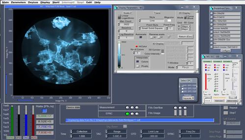
Fig. 5: Main panel of SPCM software, recommended configuration for
wide-field FLIM. Image Invitrogen BPAE sample, acquisition time 1 minute.
The count rates are displayed on the lower
left. The count rates have different meaning depending on which SPC module is
selected in the Select SPC panel. If module 1 is selected the Sync rate is
the reference pulse frequency from the laser. The other bars are the photon
rates in the at the CFD input, in the TAC, and in the ADC of the
time-measurement module. For wide-field FLIM, we recommend not to exceed a
photon rate of 1 MHz. This can cause detector saturation in bright parts of the
image, or result in a large fraction of unmatched events (unmatched time and
position information) and, consequently, loss of photons. If M2 or M3 are
selected the Sync and CFD rates show the event rates in the X1 / X2
and Y1 / Y2 position channels. All rates should be approximately the
same as the CFD rate in M1.
System Parameters
The SPCM system parameter panel with the
recommended settings is shown in Fig. 6, left. Operation mode is Wide-Field
FLIM. Stop T is not set - the measurement is started and stopped by the
operator. ADC resolution is 1024. That means, decay curves of 1024 time
channels are recorded in the pixels. Image pixels Y and Image Pixels Y is 512,
corresponding to an image of 512 x 512 pixels. The pixel number can
be increased to 1024 x 1024 to obtain larger over-sampling factors
as they are commonly used in microscopy.
To associate the events recorded in the
three SPC‑150N modules to the correct photons the modules must be started
synchronously, and be operated from the same master clock. The definitions are
shown in Fig. 6, right.
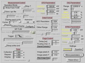
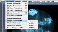
Fig. 6:
System Parameters (left) and definition of Trigger Master and Master Clock
function (right)
System-specific parameters are defined
under More Parameters, see button in the system parameter panel, lower right.
These parameters control the conversion of the times measured between the X1
and X2, and the Y1 and Y2 signals into spatial information. We recommend not to
change these settings.
Running a Measurement
To run a measurement, click Enable
Outputs in the DCC-100 panel. Open the shutter (green button), and select an
appropriate laser power (left slider). If you control the detector operating
voltage via the DCC-100, select also the correct voltage. We recommend to set
the voltage only once and then use Lock Con 3 Setup in the Options. The
software then automatically uses the right voltage everytime it starts.
With the parameters shown above the system
starts acquiring photons when the Start button is clicked. It continues to do
so until the operator clicks the Stop button. Intermediate results are
displayed in intervals of Display Time, i.e. 1 second with the parameters
shown in Fig. 6.
A fast preview is run when the Repeat and
the Stop T buttons are activated (Fig. 5, lower right) or Fig. 6, left,
Measurement Control. With the parameters selected the system runs 1-second
measurements and displays the results periodically. The Fast Preview function
is an excellent way to select the desired laser power, sample position, and
focal plane.
Results
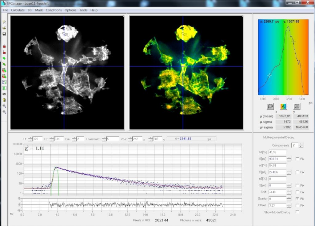
Data Analysis was performed by SPCImage [2]
in the usual way, see Fig. 7. An intensity image build up from the TCSPC data
is shown left, a lifetime image is shown right. A decay curve for the pixel at
the cursor position is shown at the bottom. The decay curve is clean, without
optical or electrical reflections. The residuals (shown below the decay curve)
confirm the good quality of the temporal data.

Fig. 7: Data
analysis by SPCImage. Same data as shown in Fig. 5, 512x512 pixels, 1024 time
channels per pixel. Sample Invitrogen BPAE cells.
A lifetime image at larger scale is shown
in Fig. 8, left. The image was recorded with 512 x 512 pixels. This
is more than the detector / TCSPC combination resolves. Fig. 8, right, shows a
zoom into an area near the centre of the image. It can be estimated that the
effective spatial resolution of the detector/TCSPC combination is about
250 x 250 pixels. This corresponds to about 160 µm on the
cathode of the detector.
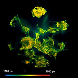
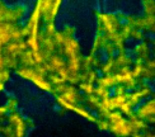
Fig. 8: Left:
Wide-field FLIM image analysed with the parameters shown in Fig. 7. Right:
Digital zoom into an area near the centre of the image.
The temporal instrument response function
(IRF) of the detection system for different spots at the photocathode is shown
in Fig. 9. To avoid saturation of the channel plates by high local intensity
the IRF measurement was performed at a count rate of no more than 70 kHz.
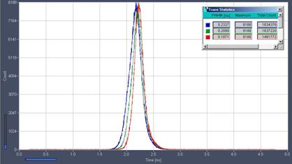
Fig. 9:
Temporal instrument response function (IRF) for different x positions on the
photocathode
The full-width at half-maximum (FWHM) is 187
to 233 ps. There is a slight change in the IRF shape and position with the
position on the photocathode. The shift in the first moment of the IRF is about
75 ps. There are two reasons for this shift. The first one is that the
timing signal is derived from one side of the microchannel plate. Therefore
there is a non-zero propagation delay from the detection position to the output
signal line. The second one is that there is a systematic variation in the
shape of the electrical single-photon pulse with the detection position. The
shape variation causes a shift of the zero-cross point in the CFD. Both effects
result in a dependency of the IRF on the spatial position at which the photons
are detected. A shift in the first moment of the IRF induces a shift of
approximately the same size in the calculated fluorescence lifetimes. For the
FLIM data analysis we therefore used a floating IRF [2].
Discussion
The setup described in this application
note is a fully functional wide-field TCSPC FLIM system. The operation of the
system is fully integrated in the bh SPCM TCSPC software. Data analysis is
performed in the usual way by SPCImage. The data obtained with the system
feature good time resolution, and reasonably good spatial resolution. Compared
to scanning systems [2, 4], the system does, however, suffer from the general
problems of wide-field imaging: Missing suppression of out-of-focus
fluorescence and lateral scattering, and contamination by fluorescence and
scattering in the optics [5]. These effects restrict the use of the system to
thin samples with low internal scattering. Possible applications are TIRF and
light-sheet microscopy which are inherently wide-field [6]. There may also be
applications which forbid point scanning because of system complexity or
temporarily high excitation power. Another application may be combined
FLIM/PLIM with phosphorescence markers of millisecond lifetimes [7]. Such long
lifetimes require extremely slow scanning but do not pose problems to
wide-field FLIM. Wide-field FLIM may also by useful for recording fast
physiological processes in cells, see, for example [8]. The time resolution for
the physiological effect then would not be limited by the scan rate.
References
1.
W. Becker, Advanced time-correlated single-photon counting techniques. Springer, Berlin, Heidelberg, New York, 2005
2. W. Becker, The bh TCSPC handbook. 9th edition, Becker & Hickl
GmbH (2021), available on www.becker-hickl.com
3. W. Becker, L. M. Hirvonen, J. Milnes, T. Conneely, O. Jagutzki, H.
Netz, S. Smietana, K. Suhling, A wide-field TCSPC FLIM system based on an MCP
PMT with a delay-line anode. Rev. Sci. Instrum. 87, 093710 (2016)
4. Becker & Hickl GmbH, DCS-120 Confocal Scanning FLIM Systems, 6th
ed. (2015), user handbook. www.becker-hickl.com
5.
W. Becker, V. Shcheslavskiy, H. Studier, TCSPC FLIM with Different
Optical Scanning Techniques, in W. Becker (ed.) Advanced time-correlated
single photon counting applications. Springer, Berlin, Heidelberg, New York (2015)
6. Liisa M. Hirvonen, Wolfgang Becker, James Milnes, Thomas Conneely,
Stefan Smietana, Alix Le Marois, Ottmar Jagutzki, Klaus Suhling, Picosecond
wide-field time-correlated single photon counting fluorescence microscopy with
a delay line anode detector. Appl. Phys. Lett. 109, 071101 (2016)
7. Becker & Hickl GmbH, Simultaneous Phosphorescence and
Fluorescence Lifetime Imaging by Multi-Dimensional TCSPC and Multi-Pulse
Excitation. Application note, www.becker-hickl.com
8. Becker & Hickl GmbH, bh FLIM Systems Record Calcium Transients
in Live Neurons. Application note, www.becker-hickl.com
Contact:
Wolfgang Becker
Becker & Hickl GmbH
Berlin, Germany
becker@becker-hickl.com