High-Resolution LIDAR with the SPC-QC-104
Wolfgang
Becker, Thomas Meures, Becker & Hickl GmbH
Abstract: We describe LIDAR with a bh SPC-QC-104
TCSPC module and a bh BDS‑SM 640‑nm picosecond diode laser.
The beam of the laser was directed to a distant target, photons scattered back
from the target were collected by a Meade LX90 20-cm telescope, detected
by a bh PMC-150-20 PMT module, and recorded by the TCSPC device. Using a laser
pulse repetition rate of 250 kHz and no more than 10 µW of
average power we obtained a clean backscattering signal from a tree 160 meters
away. By increasing the pulse repetition rate to 50 MHz, we were able to
detect fluorescence decay curves from the chlorophyll in the leaves.
Basic Principle
The distance to a distant objet can be
measured by sending laser pulses to it, detecting light reflected or scattered at
the object and determining the propagation time of the pulses to the object and
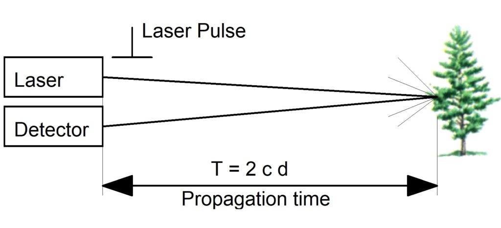
back. The technique is called Light Detection and Ranging, or LIDAR. The
principle is illustrated in Fig. 1.
Fig. 1:
Principle of LIDAR
The intensity of the light reaching the
detector decreases with the distance of the object. For distances in the 100-m
range and above and moderate laser power the intensity quickly drops to the
single-photon level. A histogram of the photon times then shows a peak at a
time T = 2 c d after the laser pulse, see Fig. 1, right. Time-correlated
single photon counting (TCSPC) or related techniques are then the techniques of
choice [1, 2].
The instrument-response function (IRF) of a
TCSPC-based LIDAR system is given by the convolution of the laser pulse shape,
the transit-time spread function of the detector, and the electrical
instrument-response function of the TCSPC device. Even with medium-speed TCSPC
devices, medium-speed detectors, and picosecond diode lasers an IRF width below
100 ps (FWHM, full width at half maximum) or 40 ps (RMS, root mean
square) can be reached. Ultra-fast TCSPC devices with high-speed detectors can
be 5 times faster than that [1,
3].
The actual resolution of a LIDAR experiment
can be even higher. The reason is that not only one photon is used to build up
the histogram shown in Fig. 1. The standard deviation of the measured
propagation time then decreases (and the accuracy increases) with the square
root of the number of photons. For example, for a system IRF of 40 ps
(RMS) and 10,000 photons the standard deviation of the transit time becomes 0.4 ps,
and the standard deviation of the distance is 60 µm. With a resolution
that high not only the distance can be determined very accurately, but also
optical properties, such as surface texture, photon migration times within the
object, or fluorescence lifetimes the can be determined.
Experiment Setup
To demonstrate LIDAR with a TCSPC device we
used a bh SPC-QC-104 module [4]. The SPC‑QC-104 has an electrical IRF of
38 ps FWHM, or about 18 ps RMS. The advantage of the SPC-QC compared
with faster SPC-150N or 180N modules is that it can record more than one photon
within the start-stop time [4]. The possible detection of background photons
therefore does not suppress the detection of a target photon at later times. As
a light source we used a bh BDS-SM 640 nm ps diode laser. The laser was
pulsed externally at a repetition rate of 250 kHz. The average power at
this repetition rate is less than 10 µW, the pulse energy is about
40 pJ. Photons from the target were collected by a Meade LX90 (20 cm) telescope
and detected by a bh PMC-150-20 photomultiplier module attached to the eyepiece
holder. A photo of the optical setup is shown in Fig. 2.
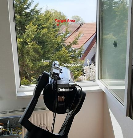
Fig. 2:
Optical setup
The low laser power and the low pulse
energy used in our setup helps avoid laser-safety problems. However, it creates
a problem with the pickup of environment light. The experiments were therefore
performed at night. Even at night, light pollution turned out to be a problem.
The pickup of ambient light was therefore reduced by a bandpass filter in front
of the detector.
Results
Distance Measurement
A result is shown in Fig. 3. Despite the
low laser power of the diode laser a clean signal was picked up from the
target. The bump on the left is from the side-lobes of the laser beam diffusely
scattered at a nearby tree, the peaks after the main peak are from trees behind
the primary target.
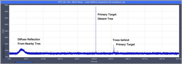
Fig. 3: LIDAR
result obtained with the setup shown in Fig. 2. Laser repetition rate
250 kHz, laser pulse energy 40 pJ.
A zoom into the data around the target peak
is shown in Fig. 4. The time of the maximum of the peak is 1070.21 ns,
corresponding to a distance of 160.53 m.
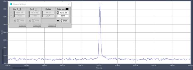
Fig. 4: Zoom into the region around the primary-target peak. The peak time
is 1070.21 ns, corresponding to a target distance of 160.53 m.
Fluorescence-Lifetime Measurement
The success in recording scattered light
from trees over a distance of more than 160 m prompted us to try recording
of fluorescence decay functions of chlorophyll over the same distance. For a
given average laser power, the intensity of fluorescence is several orders of
magnitude lower than that of scattered laser light. However, the loss in
intensity can be compensated by increasing the laser pulse repetition rate.
There is no need of low repetition rate to avoid ambiguity, as in the case of
distance measurement. The laser can therefore be run at its nominal repetition
rate of 50 MHz, effectively increasing the average power by a factor of 200.
The bandpass filter was replaced with a 680-nm long-pass filter, and the TCSPC
recording-time window decreased to 16 ns. The time-channel width was set
to 4 ps, and the number of time channels to 4096. The result was striking:
The count rate increased to about 300,000 photons per second, and fluorescence
decay curves showed up almost instantly. An example is shown in Fig. 5.
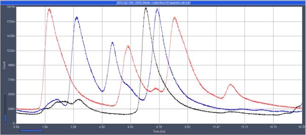
Fig. 5: Fluorescence decay curves of chlorophyll recorded from a tree
160 m away. The three curves were recorded from slightly different
locations. The laser beam illuminated several leaves simultaneously, therefore
several decay profiles are present in each curve.
Three curves (red, blue and black) were
recorded from slightly different spatial locations. Moreover, the laser beam
hit several leaves in slightly different distance. Therefore, several overlaid decay
profiles are visible in each curve.
An attempt to de-convolute a decay curve
with SPCImage NG [6] is shown in Fig. 6. The black curve of Fig. 5 was sent to
SPCImage NG, and the fit range restricted to the decay curve in the centre. A
double-exponential model and a synthetic IRF were used for the fit. The fit of
the rising edge is not perfect, probably because there are small signal contributions
from leaves in different distances. Nevertheless, reasonable decay times and
amplitudes are obtained. The decay components are shown in the insert in the
upper right of the figure.
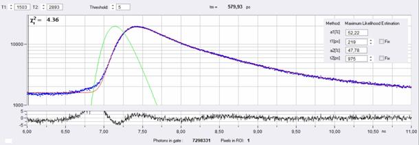
Fig. 6: De-convolution of the decay in the middle of the black curve in Fig.
5. Double-exponential model, synthetic IRF. Decay components shown in the
insert upper right. The green curve is the IRF.
The decay times of the two components are t1
= 219 ps and t2 = 975 ps, the amplitude-weighted lifetime is tm = 580 ps.
This is a short lifetime for chlorophyll. The short lifetime explains by the
fact that the leaves are fully dark adapted, and the excitation power density
is extremely low. Under these conditions, the photosynthesis channels are fully
open, and the fluorescence is quenched by photosynthesis reactions.
Summary
We described LIDAR
with a bh SPC-QC-104 TCSPC module and a bh BDS‑SM 640‑nm
picosecond diode laser. The beam of the laser was directed to a distant target,
photons scattered back from the target were collected by a Meade LLX19
20-cm telescope, detected by a bh PMC-150-20 PMT module, and recorded by the
TCSPC device. Using a laser pulse repetition rate of 250 kHz and no
more than 10 µW of average power we obtained a clean backscattering signal
from a tree 160 meters away. By increasing the pulse repetition rate to
50 MHz, we were able to detect fluorescence decay curves from the
chlorophyll in the leaves. The results show that TCSPC-based LIDAR not only
delivers distances to remote objects but also reveals information on the objects
themselves.
References
1.
W. Becker, The bh TCSPC Handbook, 9th ed. Becker
& Hickl GmbH (2021)
2.
W. Becker, Advanced time-correlated single-photon counting techniques. Springer,
Berlin, Heidelberg, New York, 2005
3.
Becker & Hickl GmbH, The bh TCSPC Technique.
Principles and Applications. Available on www.becker-hickl.com.
4.
SPC-QC-104 3-channel TCSPC FLIM Module, user
manual. Available on www.becker-hickl.com.
5.
BDS-SM Series ps Diode Lasers, extended data
sheet. Available on www.becker-hickl.com.
6.
SPCImage Data Analysis, in W. Becker, The bh
TCSPC Handbook, 9th ed., Becker & Hickl GmbH (2021)
zMHM
Contact:
Wolfgang Becker
Becker & Hickl GmbH
Berlin, Germany
Email: becker@becker-hickl.com