We demonstrate fluorescence-lifetime based imaging of membrane potentials in cells with a voltage sensitive dye. We estimate the number of photons per pixel required for a given standard deviation of the membrane potential, show ways of improving the accuracy and compare the predictions with real measurement data. In the experiments described, we achieved a standard deviation of the membrane voltage on the order of a few mV.

Related Applications

TCSPC FLIM

Related Application Notes

Download PDF

Measurement of Membrane Potentials in Cells by TCSPC FLIM

Wolfgang Becker, Axel Bergmann, Becker & Hickl GmbH, Berlin, Germany

Abstract: We demonstrate fluorescence-lifetime based imaging of membrane potentials in cells with a voltage sensitive dye. We estimate the number of photons per pixel required for a given standard deviation of the membrane potential, show ways of improving the accuracy and compare the predictions with real measurement data. In the experiments described, we achieved a standard deviation of the membrane voltage on the order of a few mV.

Membrane Potential

Cells have concentration gradients of ions across their membranes. These gradients produce a voltage over the membrane which is characteristic of a number of fundamental cellular processes [1]. Unfortunately, techniques for precise measurement of membrane potentials are rare. Patch-clamp techniques are highly invasive and do not deliver spatially resolved data. Optical methods based on the fluorescence intensity exist but are not quantitative. Ratiometric intensity imaging has not yet resulted in quantitative results. A promising solution is FLIM with a voltage-sensitive dye [10]. FLIM is intrinsically ratiometric and thus able to deliver quantitative results [3, 12]. 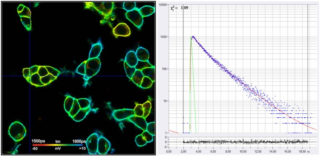The figure below shows a FLIM image of cells loaded with VoltageFluor VF2.1.Cl [10, 11].

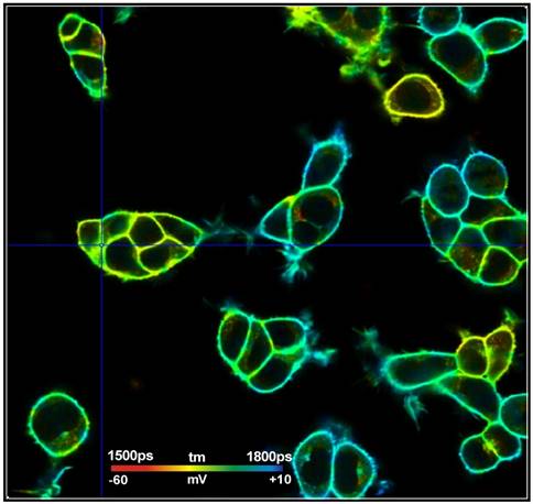
Fig. 1: FLIM image of HEK cells loaded with a voltage-sensitive dye. Data courtesy of Susanna Yaeger-Weiss, University of Berkeley

The FLIM format is 512 x 512 pixels with 1024 time channels per pixel. The data were recorded by a standard Becker & Hickl (bh) TCSPC System on a Zeiss LSM 980 laser scanning microscope. The system contains two parallel SPC-150NX TCSPC/FLIM modules [2, 7, 8] with HPM-100-40 hybrid detectors [2]. For excitation, the system contains a bh 'Laser Hub' with four ps diode lasers [9].

The excitation wavelength used for the measurement was 445 nm, the detection wavelength 525 nm to 550 nm. The raw data were processed by bh SPCImage NG data analysis software. Maximum-Likelihood Estimation (MLE) with a double-exponential incomplete-decay model was used to fit the decay data. The synthetic IRF of SPCImage was used for deconvolution and a double-exponential model was used to fit the data. The image was colour-coded with the amplitude-weighted lifetime, tm [4, 5]. A binning radius of 6 was used to obtain a high signal-to-noise ratio of tm, please see section 'Binning'.

A decay curve at the cursor position is shown in Fig. 2. The blue dots represent the photon numbers in the subsequent time channel, the red curve is the IRF, the red curve represents a fit with a double-exponential decay model. The decay parameters are shown upper right.

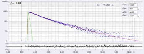
Fig. 2: Decay curve at cursor position of Fig. 1.

Both the FLIM image and the decay curve are proof of the high quality of the data. A near-perfect fit of the decay data was obtained. The tm image clearly shows heterogeneity of the lifetime, which means that different cells have different membrane potentials.

Lifetime-Voltage Calibration

Calibration data for VF2.1.Cl are given in [10]. The sensitivity, s, is 3.5±0.08 ps/mV, and the zero-mV lifetime, t₀, is 1.77±0.02 ns. Within the calibration range of -80 mV to +80 mV the lifetime-voltage relation is linear. A calibration curve is shown in Fig. 1.

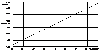
Fig. 3: Calibration curve, amplitude-weighted lifetime, tm, vs. membrane potential, V_m. Redrawn from [10].

With these calibration values the lifetimes in Fig. 1 were transformed into voltage values, see V_m values under the colour bar at the bottom of the image.

Standard Deviation of Vm

With the calibration values above, the standard deviation of Vm in dependence of the number of photons per pixel, or, reversely, the number of photons needed to reach a given standard deviation of the voltage can be estimated.

The standard deviation, s_t, of the fluorescence lifetime, t, obtained from a decay curve with a number of photons, N, is

(1)

s_t is the accuracy that can be achieved under ideal conditions. 'Recorded under ideal conditions' means that the decay data are recorded at a temporal resolution much higher than the fluorescence lifetime, without noticeable counting background, and with the entire decay curve being in the observation-time-interval. A carefully operated TCSPC FLIM system comes very close to these conditions [2, 3, 6]. However, to obtain the ideal s_t from the decay data also the FLIM data analysis had to perform at ideal efficiency. Unfortunately, this is not entirely possible. The decay profile of VF2.1.Cl in the cells is double-exponential, and the calibration values given in [10] are amplitude-weighted lifetimes, t_m. Amplitude-weighted lifetimes can only be obtained by a fit procedure, and a fit procedure does not deliver the ideal s_t. The resulting loss in accuracy is described by the 'Photon Efficiency', E. The Photon Efficiency is the ratio of the photon number an ideal recording and analysis system would need to reach a given accuracy to the photon number the real system needs. The standard deviation obtained with the real system, s_treal, is then

(2)

The standard deviation, s_V, of the measured membrane potential around the zero-voltage point, t₀ , is

(3)

and the number of photons required to reach a given s_V is

(4)

For the MLE fit of SPCImage NG the photon efficiency, E, is about 0.7 [6]. With E= 0.7, the number of photons, N, versus the desired standard deviation, s_V, of the membrane voltage is as shown in Fig. 4.

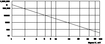
Fig. 4: Number of photons per pixel, N, needed for a desired standard deviation, s_V, of the membrane voltage, V_m

As expected, the number of photons increases with the square of the reciprocal standard deviation of the voltage. For a standard deviation of 10 mV N=3400 photons are required. This is well within the reach of a normal FLIM measurement. However, below that the photon number becomes unrealistically high. For example, for a standard deviation of 2 mV more N = 85,000 photons per pixel are required. Nevertheless, we will show how photon numbers in this range, and, consequently, V_m accuracies better than 10mV can be achieved.

Binning of the Decay data

Attempts to increase the number of photons by increasing the excitation power usually fail because the imaging procedure is no longer non-invasive. A substantial fraction of the fluorophore photobleaches. Photobleaching produces radicals, and the radicals destroy the cells or at least impair their metabolic function. Extending the acquisition time to acquire more photons is, in principle, possible. bh FLIM system are so stable that acquisition over hours is possible [2]. However, also here photoreactions set a limit to the acquisition time. Moreover, motion in the sample can cause blurring of the images over longer periods of time.

A substantial increase in photons numbers can be obtained by the overlapping-binning function of SPCImage NG. The function leaves the number of pixels of the image unchanged but, for each pixel, combines the decay data of several pixels around it into the decay analysis. The procedure is justified by the fact that, for best spatial resolution, microscope images are oversampled. That means the point-spread function is sampled by (typically) 5x5 pixels or more. The decay information within these pixels is highly correlated. Overlapping binning therefore does not impair the spatial resolution of the lifetime data. Please see [4, 5, 6] for details. In case of membrane-potential imaging with VF2.1.Cl the binning function is particularly efficient. The fluorophore strictly adheres to the cell membranes. There is virtually no fluorescence outside the membranes. Binning, even with large binning area, therefore does not mix unwanted decay components from inside or outside the cells into the decay data of the membranes. Mixing decay data of different pixels can occur only along the membrane. However, this is rarely a problem because there are no abrupt changes in the fluorescence lifetime within one and the same cell. The binning principle is illustrated in Fig. 5.

Fig. 5: Binning of decay data in SPCImage. Decay data of every pixel are combined with data from a larger area around. Binning areas for adjacent pixels (binning radius bin=6) indicated in the image.

Experimental Results

Decay curves from an arbitrarily selected pixel on a cell membrane are shown in Fig. 6. From left to right, the binning radius is 1, 6, and 10. It can be seen how the effective photon number increases with the binning radius. Fig. 7 shows Lifetime / Vm images for binning radius 1 (top) and binning radius 6 (bottom). Histograms of the lifetime, tm, for three different regions of interest (ROIs) are shown on the right. For bin = 1 the histograms are broad and overlapping. For bin=6 the histograms become clearly separated, revealing real V_m heterogeneity between different cells.

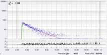
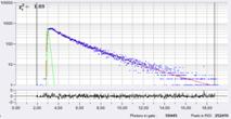
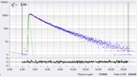
Fig. 6: Decay curves of an arbitrarily selected pixel on a cell membrane for different binning radius in SPCImage. Left: Bin=1, N=4621, Middle: Bin=6, N=59,445, Right: Bin=10, N=133,404. Note logarithmic scale. The expected standard deviation of V_m is 8.5 mV, 2.3 mV, and 1.6 mV, respectively.

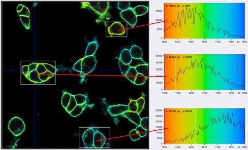
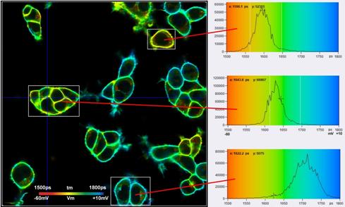
Fig. 7: FLIM images and tm histograms in three different regions of interest. Upper image: Binning radius bin=1. The histograms are broad and overlapping. Lower image: Binning radius bin=6. The histograms are clearly separated, indicating real V_m heterogeneity in the sample. Same data as Fig. 1, analysis with SPCImage NG, MLE fit. t_m range is 1500 ps to 1800 ps, V_m range is -65 mV to +10 mV.

Fig. 7 shows that TCSPC FLIM delivers membrane potentials at unprecedented resolution. Nevertheless, the histograms in the regions of interest are broader than predicted by equations 2 and 3. With a number of photons, N, of about 60,000 in the binning area, E = 0.7, and t_m » 1.7 ns, s_t should be about 8.3 ps, and s_V about 2.3 mV. However, the t_m histograms in the ROIs have a width of about 40 ps, 45 ps, and 70 ps (full width at half maximum). This translates into a s_t of about 17 ps, 19 ps and 30 ps, and a s_V of about 4.8 mV, 5 mV, and 8.5 mV. That means the standard deviations are about twice as large as expected. Based on the analysis results of countless other FLIM data [6] we can exclude that the equations (2) and (3) are wrong, or that E is substantially lower than 0.7. The only explanation that remains is that there is still Vm heterogeneity within the individual ROIs. This indeed seems to be the case. Fig. 8 shows the cells in the selected ROIs with individually adjusted t_m and V_m scale. At this scale, non-random variation in the lifetime and the membrane voltage shows up which is not apparent in Fig. 7, bottom. We therefore believe that the V_M resolution is higher than indicated by the width of the tm histograms and indeed close to the expected value s_V= 2.3 mV.

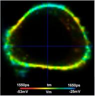
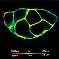
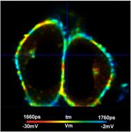
Fig. 8: Cells in the regions of interest marked in Fig. 7. Individually adjusted lifetime / voltage scale.

Conclusions

FLIM-based measurement of membrane potentials delivers the voltage across the membrane at a standard deviation of a few mV. As shown in equation (3) the accuracy increases with the effective number of photons per pixel and the photon efficiency, E, of the recording technique and the decay analysis. TCSPC FLIM in combination with MLE analysis delivers maximum N and near-ideal E. It is thus the method of choice for membrane-potential measurement.

Equation (3) further shows that the accuracy increases with the ratio of the lifetime, t₀, and the voltage sensitivity, s, of the fluorophore. Candidates for voltage-sensitive probes should therefore not only be selected for high s but also for short lifetime.

Of all parameters affecting the voltage resolution the effective number of photons per pixel, N, has the largest influence. Attempts to increase N by higher excitation power or higher fluorophore concentration usually fail. Excessively high excitation power results in photobleaching, creation of radicals, changes in the cell metabolism, and, finally, cell damage. Increasing the fluorophore concentration in the cell membrane, if not by itself toxic to the cell, most likely leads to coupling of the excited states of different molecules and to unpredictable lifetime changes.

A massive increase of the effective N is obtained by the overlapping binning function of SPCImage NG. The function exploits the fact that microscopy images are oversampled and thus overlapping binning has little effect on the spatial resolution of the lifetime analysis. For the VF2.1.Cl probe binning is further supported by the fact that it binds almost quantitatively to the membranes. The decay functions at the membrane are therefore not contaminated by out-of-membrane fluorescence, so that a large binning radius can be used. Practically achieved improvements by overlapping binning are on the order of 16 in photon number and four in voltage accuracy.

Of course, the photon number, N, per pixel can also be increased by decreasing the number of pixels in the raw data. However, reducing the number of pixels reduces the spatial resolution and is thus inferior to overlapping binning in SPCImage. Raw data should always be recorded with a pixel number that adequately resolves the spatial structure of the sample.

Another useful option for accuracy improvement is to increase the acquisition time. The data shown in this document were recorded within an acquisition time of 147 seconds, or about 2.5 minutes. This may sound a lot when compared with other FLIM applications. Nevertheless, an increase to 5 minutes or even 10 minutes appears feasible. The standard deviation of V_m would then improve by a factor of 1.4 and 2, respectively. The bh TCSPC systems are stable enough to run the acquisition for 10 minutes or more. Whether the cells retain their spatial position and their metabolic state over such a period of time must be proofed by future experiments.

Attempts to increase the photon efficiency, E, of the data analysis are not promising. In principle, E could by increased to 1 by using first-moment analysis [5, 6]. However, first-moment analysis delivers only the lifetime of a single-exponential approximation of the fluorescence decay. This can cause problems with multi-exponential decay functions and would mean that new calibration data had to be created. Moreover, E is already 0.7. Increasing it to 1 would only yield a minuscule improvement in accuracy.

Finally, it should be mentioned that massive changes in the number of recorded photons and in the photon efficiency can be induced by unfavourable recording conditions. Correct focusing, correct pinhole alignment in confocal systems, high numerical aperture of the microscope lens, and suppression of leakage of room light into the detection light path are mandatory. Please see [6] for details.

It should be noted that the considerations in this paper apply only to the error induced by photon statistics. They do not include systematic effects, such as timing stability of the TCSPC electronics or timing stability of the laser. The timing stability of the bh TCSPC/FLIM modules is better than one ps (standard deviation) [2]. The timing stability of the entire FLIM system, including bh ps diode lasers is better than 5 ps. Part of this shift is compensated by the data analysis. It can therefore be concluded that the systematic error is no larger than a few ps, or about 1 mV in membrane potential.

Another potential error is the uncertainty of the calibration curve in different molecular environment. Differences for different HEK293T cells were found as large as 70 ps in lifetime or 20 mV in membrane potential [10]. This is 10 times more than the statistical error. Interestingly, the differences in the calibration curves are on the same order as the differences between individual cells in Fig. 7. These cells are of absolutely similar type, have grown in the same medium, and contain comparable concentrations of the VF2.1.Cl. It is hard to believe that VF2.1.Cl behaves differently in these cells. It is rather possible that the reason of the different V_m is not a different t_m-V_m characteristics of the probe but different metabolic state of the cells. If this is correct different metabolic state may also account for the differences in the calibration curves. Measurements of the metabolic state via the the amplitudes of the decay components of NAD(P)H [2] may help answer this question.

Acknowledgement

We acknowledge the work of Julia R. Lazzari-Dean, Anneliese M.M. Gest, Evan W. Miller, and Susanna Yaeger-Weiss of University Berkeley who developed the technique of FLIM-based imaging of membrane potentials with voltage-sensitive dyes. Especially, we thank Susanna Yaeger-Weiss for recording top-quality FLIM data of VF2.1.Cl-stained HEK cells.