Bigger and Better Photons:
The Road to Great FLIM Results
Wolfgang Becker, Becker & Hickl GmbH
Abstract: These pages are an attempt to help
existing and future users of the bh FLIM technique obtain the best possible
results from their FLIM experiments. The first part of the brochure explains
the principle of TCSPC FLIM, and gives an impression of the photon
distributions recorded. It shows that the signal-to-noise ratio of the measured
lifetimes depends, in first order, on the number of photons recorded. The
following sections focus on optimising the photon number without increasing the
photostress imposed to the sample. We discuss the influence of excitation
power, acquisition time, collection efficiency, numerical aperture, focusing
precision, alignment accuracy, and detector efficiency. The next section
concentrates on photon efficiency. It considers TCSPC timing parameters,
counting background, number of pixels, the influence of the instrument-response
function, and the challenges of multi-exponential decay functions. The last
section is dedicated to data analysis. All conclusions made in this brochure
are demonstrated on real measurement data recorded under realistic conditions.
What makes a great FLIM image? Well, it
should have perfect spatial resolution, it should be recorded into a
sufficiently high number of pixels, it should have high contrast, low
background, no out-of-focus blur, and it should display the fluorescence
lifetime at a high signal-to-noise ratio. Just as the image shown below. An
experienced FLIM user will probably add that just recording the fluorescence
lifetime is not enough, and the entire decay function should be recorded in
every pixel.
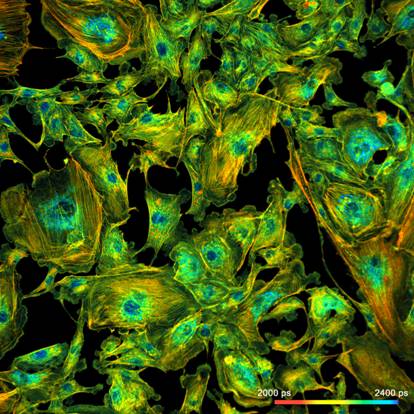
Fig. 1: FLIM
image of a BPAE sample. 2048 x 2048 pixels, decay functions recorded into 256
time channels. bh DCS‑120 confocal FLIM system, bh SPCImage FLIM data
analysis software.
Why do FLIM images published in scientific
papers rarely look like the image above? There is actually no reason for that.
All that has to be done is to use perfectly aligned optics, the right
microscope lens, perfect focusing, the right excitation and detection
wavelengths, the right detector, and a little bit of patience. Some
comprehension of the signal-processing principles of FLIM may be helpful as
well. This is something every FLIM user can achieve.
This article shows what is important to
obtain great FLIM results. Most of the advice given on these pages will be
trivial. However, it is just the sum of these trivial things that makes the
difference between a mediocre lifetime image and a perfect FLIM result.
The road to perfect FLIM results starts
with the understanding that a TCSPC FLIM result is a photon distribution [1]. The
basic principle of the recording process is shown in Fig. 2.
The sample is scanned by a high-frequency
pulsed laser beam, single photons of the emitted fluorescence light are detected,
and the arrival time, t, of each photon in the laser pulse period is determined
by the TCSPC system. In parallel, the TCSPC system determines the spatial
coordinates, x,y, of the laser beam in the moment of the photon detection. From
these data, the distribution of the photons over the spatial coordinates and
the times of the photons is built up. This photon distribution is the desired
lifetime image: It is a data array of x × y pixels, each of which contains a
fluorescence decay function in a large number of consecutive time channels. See
Fig. 2, right. A detailed description of the recording process and its various
extensions can be found in [2].
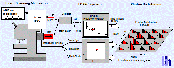
Fig. 2: Principle
of TCSPC FLIM
Fig. 3 gives an impression of the photon
distribution recorded by FLIM. The figure shows an image area of 8 horizontal x
128 vertical pixels. Each pixel has 256 time channels, containing decay data of
this pixel. Of course, a real FLIM image has a much higher number of pixels.
FLIM formats of 512 x 512 pixels with 256 to 1024 time channels are used
routinely, and formats of 2048 x 2048 pixels with 256 time channels have
been demonstrated [2].
To an inexperienced user the distribution
shown in Fig. 3 may look very 'noisy': The fluorescence decay in the individual
pixels can barely be seen. Of course, the 'noise' is not caused by any noise of
the detector or the TCSPC electronics. It is simply an effect of photon
statistics. The reason that the noise is so high is that the photons are
distributed over a large number of pixels and time channels. Consequently, the
number of photons in the individual pixels, and, especially, in the individual
time channels if each pixel is low. So, how can the 'noise' in the photon
distribution be reduced? The only way is to record more photons, see Fig. 4.
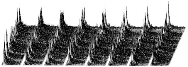
Fig. 3: The photon distribution of TCSPC FLIM. The figure represents an
image area of X × Y = 8 × 128 pixels. Each pixel has 256 time channels, each
containing the photons at consecutive times within the fluorescence decay.
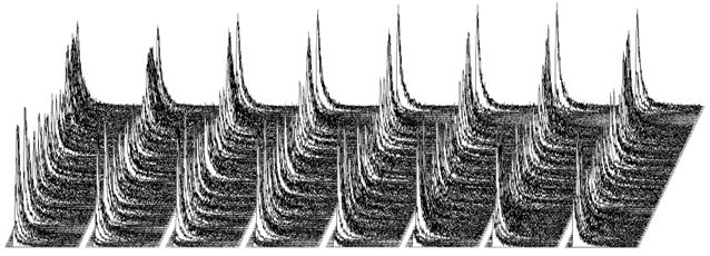
Fig. 4: The same photon distribution as shown in Fig. 3, but after
recording 10 times more photons. The signal-to-noise ratio is 3.1 times higher,
and the fluorescence decay curves in the individual pixels stand out clearly.
What is the signal-to-noise ratio of a fluorescence
lifetime derived from such data? We obtain the answer from a simple
gedankenexperiment.
By definition, the fluorescence lifetime, t, is the average
time a molecule stays in the excited state. When a molecule gives off a photon
it means that it returned from the excited state. The FLIM system detects the
individual photons and determines their times, t, after the excitation pulse,
see Fig. 5, a and b. When the FLIM system detects a large number of such photons
their average arrival time after the excitation pulse is the average time of
the molecules in the excited state and thus the fluorescence lifetime, see Fig.
5 c. Although the FLIM hardware normally does not calculate the average arrival
time directly, it is implicitly present in the photon distribution.
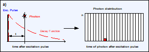
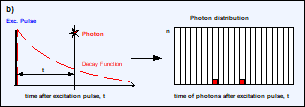
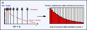
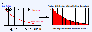
Fig. 5, a and b: Detection of photons and buildup of the photon distribution
over the time after excitation, t. c: Photon distribution after the detection
of N photons. The average arrival time after the excitation, <t>, is the
fluorescence lifetime, t. d: The standard deviation, st, of the arrival times, t, is t. The standard deviation, st, of the average
arrival times is t / SQRT(N).
What is the signal-to-noise ratio of the
average arrival time? The standard deviation, st, of the arrival time of the individual
photons is identical with the fluorescence lifetime, t, itself. This is a
property of the exponential function. If we average the arrival times for a
number of photons, N, the standard deviation, st, of the result decreases
with the square root of N, see Fig. 5, d. The signal-to-noise ratio, i.e. the
ratio of t divided by its standard deviation, st after the detection of N photons is
therefore:
SNRt = t / st = SQRT (N)
That means the standard deviation at which
the fluorescence lifetime can be obtained is simply the square root of the
number of photons in the decay curve [20]. This is a remarkable result in
several respects. First, the signal-to-noise ratio for the pixel lifetime is
the same as for the pixel intensity. This invalidates the widespread opinion
that FLIM needs more photons (and thus more acquisition time) than steady-state
imaging. Second, the signal-to-noise ratio depends only on N. In
particular, is does not depend on the number of time channels into which the
fluorescence decay is recorded. In other words, you can increase the number of
time channels to improve the time resolution or to reduce sampling artefacts
without compromising the signal-to-noise ratio. Third, because the SNR depends
on N only, the only way to increase the lifetime accuracy is to increase N.
That means you either have to decrease the number of pixels - which you
normally don't want - or record more photons. Getting these photons recorded is
the key to a good FLIM result, and it is the subject of the next section.
As explained above, the fluorescence
lifetime of a single-exponential decay (or of a single-exponential
approximation of the decay) can be obtained by calculating the average arrival
time of the photons. If the individual arrival times of the photons are not
available the average arrival time can be obtained from the complete photon
distribution by calculating the 'First Moment', M1 [21]:
The time, t, in the above equation is the
time of the photons in the observation time interval of the FLIM system, not
the time after the excitation pulse. Therefore, the time of excitation (in
practice the first moment of the IRF) has to be subtracted to obtain t:

The method is illustrated in Fig. 2. The
blue dots are the photon numbers in the individual time channels, the green
curve is the IRF, the red curve is the hypothetical fluorescence decay function
calculated by convoluting an exponential function, e-t/t, with the
IRF.
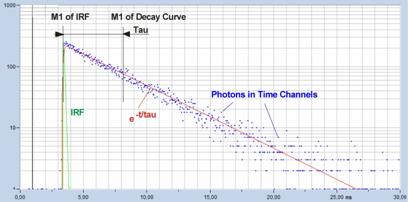
Fig. 6: First-moment calculation of
fluorescence lifetime. The lifetime is the difference of the first moment of
the fluorescence and the first moment of the IRF.
The first-moment technique delivers
single-exponential decay times at an ideal signal-to-noise ratio. However, it does
not deliver the parameters of multi-exponential decay functions, and it does
not deliver correct decay times if the recording contains background counts or if
only a part of the decay functions is in the observation-time interval of the
TCSPC system. Therefore it has almost entirely been replaced by curve-fitting
techniques. Nevertheless, the first moment technique has its benefits: It works
reliably at very low photon numbers, it is suitable for fast lifetime
determination in online-FLIM applications, and, most importantly, it provides a
way to estimate the signal-to-noise ratio of FLIM both under ideal and
non-ideal conditions. We will make use of this capability in later sections of
this brochure.
An experimental verification of the SQRT
(N) relation is shown in Fig. 7. A dye solution was scanned with different
acquisition time in order to obtain FLIM images containing about 200, 1600, and
9000 photons per pixel. Typical decay curves are show in the top row of Fig. 7.
The second row shows histograms of the fluorescence lifetime in the individual
pixels, as it is obtained by first-moment analysis. The st values and the s / t = SNR values
are indicated in the histograms. As can be seen from these values, s / t is indeed very
close to SQRT (N). The bottom row of Fig. 7 shows histograms of the lifetimes
obtained by an MLE (maximum-likelihood estimation) fit. The histograms of the
lifetime obtained from the MLE fit are a bit broader than those from the moment
analysis. But also the MLE results are close to the ideal SNR of SQRT (N).
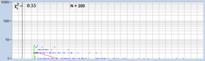
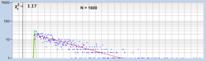
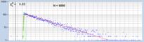
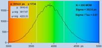
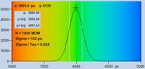
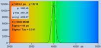
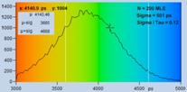
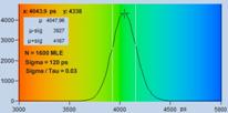
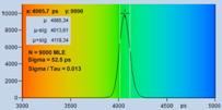
Fig. 7: Verification of the SQRT (N) relation. Top row: Decay curves from
single pixels of FLIM data from a Rhodamine 110 dye solution. Left to right: N
= 200 photons, N = 1600 photons, N = 9000 photons. Second row: Histograms of
the lifetimes obtained by first-moment analysis. Bottom row: Histograms of the
lifetimes obtained by MLE analysis.
The fact that a photon was detected does
not necessarily mean that it efficiently contributes to the accuracy of the
lifetime measurement. It can be lost by unfavourably selected timing parameters
in the TCSPC module, its detection time can be impaired by uncertainty in the
detector transit time, or there may be photons from background signals which
add unwanted noise to the photon distribution. In all these cases the SNR of
the obtained lifetimes becomes smaller than the ideal value, SQRT(N). The
situation can be described by a 'Photon Efficiency', E. The reciprocal of E
tells how many photons the non-ideal system needs in comparison to the ideal system
to reach the same signal-to-noise ratio. Since the SNR scales with the square
root of the photon number the photon efficiency can also be written
E = (SNRreal
/ SNRideal)2
The photon efficiency, E, is the square of
the 'Figure of Merit' that is sometimes used to compare the efficiency of
different lifetime-measurement techniques [13, 19]. A correctly configured TCSPC system
working under optimal conditions has a photon efficiency close to one. Reaching
the ideal photon efficiency will be the subject of section 'Maximising the
Photon Efficiency'.
When a FLIM user wishes to increase the
photon rate the first idea is usually to increase the excitation power. This is
certainly an efficient way to get more photons. However, it is not always a useful
way to obtain better FLIM results. FLIM is usually performed on samples with
low fluorophore concentration. The reason is that molecular effects can only be
seen if the fluorophore itself does not have noticeable effects on the
viability of the cells or on their metabolic functions. In addition, the
fluorophores may have low quantum efficiency. At increased excitation power the
molecules have to perform more excitation-emission cycles, with the result that
photobleaching, formation of radicals, laser-induced lifetime changes, photodamage,
or even utter destruction of the sample occurs. The imaging process is then no
longer non-invasive, and the FLIM results become meaningless. The options of
increasing the laser power are therefore limited [11]. A few examples of
invasive effects are shown in Fig. 8.
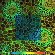
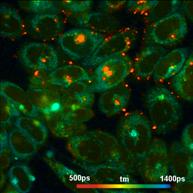
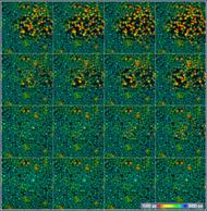
Fig. 8: Left: Convallaria image, region in the centre scanned with
405 nm laser. Middle: Two-photon NADH image of live cells. In the bright
red spots photodamage has occurred, revealing itself by spots of very fast
decay. Right: Temporal Mosaic FLIM of yeast cells, 2-photon excitation at
780 nm. Recording started in the element lower left, and proceeds to the
upper right of the array. Destruction starts in elements 8 and 9 and continues
until element 16.
Different than increasing the excitation
power, increasing the acquisition time usually is an option. Damage
effects are highly nonlinear. Often a sample can be scanned for a long time at
a power that is only moderately lower than the damage threshold. Therefore, the
options of increasing the photon number are indeed real. All that is needed is
patience of the experimentator. An example is shown in Fig. 9. The left image
was recorded with 1 minute acquisition time, the right one with 2 minutes. Not
surprisingly, the right image contains 2 times more photons. As expected, it also
provides a 1.4 times better SNR of the lifetime, see lifetime histograms underneath
the images.

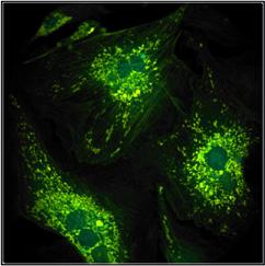
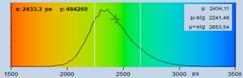
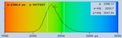
Fig. 9: Same sample imaged with
different acquisition time. Left 1 minute, right 2 minutes. Image format
512x512 pixels, 1024 time channels.
Although the dependence of the photon
number (and thus of the lifetime accuracy) on the acquisition time is trivial,
it is often not realised by FLIM users. Especially users coming from conventional
intensity-based imaging tend to stop the acquisition when a reasonable SNR of
the intensity image has been reached. However, there is a fallacy. An
intensity image starts to look good when it contains no more than a few 10
photons per pixel. The SNR of such an image may be enough to distinguish
different fluorophores but it is not enough to derive the desired molecular
information from the fluorescence lifetimes. Therefore, make sure that you run
the acquisition for a sufficiently long period of time. SPCM provides a number
of options to check the photon number during the acquisition. You can display a
decay curve in a selected pixel or in an region of interest, you can display
the photon number in the brightest pixel and in a selected pixel, and you can
display a lifetime image online. Please see Fig. 10. With these options you
should be able to decide whether the data recorded up to this point are good
enough for further analysis. If in doubt record longer.
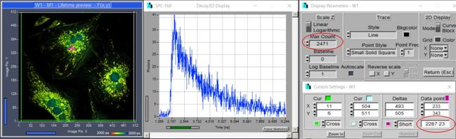
Fig. 10: SPCM functions help a user decide whether enough photons have been
recorded. Left to right: Online lifetime image, decay curve at selected
position, photon number in brightest pixel (top) and photon number at position
of data point.
It is sometimes objected that long
acquisition time is not an option when physiological changes are to be
observed. This is not entirely correct, however, if appropriate
multidimensional TCSPC techniques are used. Please see [2, 12].
The numerical aperture of the microscope
lens has a significant influence of the detection efficiency. Fluorescence is
emitted isotropically, and only a part of it is collected by the microscope
lens. Theoretically, the collection efficiency increases with the square of the
numerical aperture. That means a lens with NA = 1.25 should collect 6
times more photons than a lens with NA = 0.5. In practice the
difference is smaller because high-NA lenses have more optical elements and
less transmission. Nevertheless, the difference in collection efficiency is
striking. An example is shown in Fig. 11. Both images were recorded by
one-photon excitation and confocal detection. The left image was recorded with
an x20 air lens of NA = 0.5, the right image was recorded with an x63
oil immersion lens, NA = 1.25. The image recorded with the high-NA
lens contains three times the photons as the image recorded at low NA.
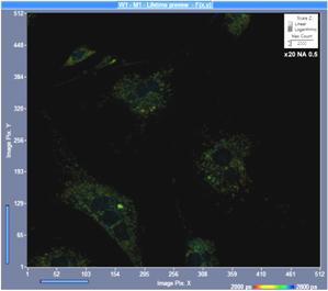
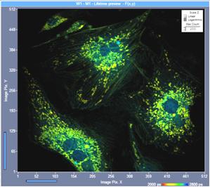
Fig. 11: FLIM image recorded with lenses of different NA, same intensity
scale. One-photon excitation, confocal detection. Left: X20 air, NA=0.5. Right:
X63 oil immersion, NA=1.25.
Focusing
Poor focusing is usually considered just a
source of sub-optimal spatial resolution. However, it has also a significant
effect on the detection efficiency. An example is shown in Fig. 12. Both images
were recorded by confocal scanning, and with the same pinhole size and the same
acquisition time. The left image is slightly defocused. Still, the image
definition is only slightly impaired. The right image is perfectly in focus. It
can easily be seen that the correctly focused image is brighter. Compared to
the defocused image, the number of photons is about 1.5 higher. The differences
are often not noticed because the FLIM system displays intensity-normalised
images. (This is done because intensities can vary over orders of magnitude)
Therefore, when you do the final focusing in the 'Preview' mode, take a few
seconds to optimise the focus with the autoscale function turned off.
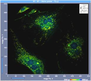
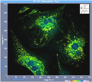
Fig. 12: Slightly defocused image (left) and perfectly focused image and
(right). Same intensity scale, one-photon excitation, confocal detection. Although
the image definition is only slightly impaired in the defocused image the
photon number is only 60 % of the photon number in the perfect image.
Image format 512 x 512 pixels, 1024 time channels.
Alignment of the Optical System
The alignment of the optical system has a massive
influence on the detection efficiency. This is especially the case for confocal
systems. Confocal alignment is extremely critical. There is virtually no
confocal system that stays in perfect alignment over a longer period of time.
An example is shown in Fig. 13. The image on the left was recorded with the
pinhole alignment slightly off. Misalignment on this level is found in almost
any confocal system. Usually, it remains unnoticed because the image definition
is virtually unimpaired. However, a comparison with the image from the
perfectly aligned system (Fig. 13, right) shows that there is a noticeable loss
in the number of recorded photons. Misalignment on a level that even causes
visible degradation in image definition can lead to a massive loss in photon
number. Efficiency degradation by an order of magnitude and more is not unusual
in these cases.
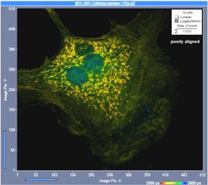
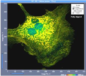
Fig. 13: Effect of confocal alignment. Left: Slightly misaligned. Right:
Perfectly aligned. Although the misalignment does not yet lead to a visible
loss in image definition it causes a loss of 50% of the photons.
Misalignment can even play a role in
multiphoton systems with non-descanned detection. Although the detection light
path of these systems is robust and rarely goes out of alignment the excitation
path is critical. The femtosecond laser of a multiphoton microscope needs to be
free-beam coupled into the scanner. This provides plenty of ways the light path
can get out of alignment. The laser is then no longer centred on the back
aperture of the microscope lens. As a result, the focus quality degrades, and
the excitation efficiency decreases. Photobleaching and photodamage do not
always decrease by the same ratio, especially if the sample has some absorption
at the fundamental wavelength of the laser. Also multiphoton systems should
therefore be re-aligned from time to time. This can easily be done by checking
the position of the laser beam in the back aperture of the objective lens and
bringing it back to the centre.
For many years, laser scanning microscopes
and, in particular, FLIM systems have been built with conventional photomultipliers
(PMTs). PMTs have large active areas, extremely low dark count rates per
square-millimeter of active area, and sufficient gain and speed to detect
single photons. The photocathodes of PMTs with conventional photocathodes have
about 20% quantum efficiency. However, not every photoelectron emitted by the
cathode enters the amplification system and delivers a useful single-electron
pulse. The net efficiency is therefore on the order of 15%. The efficiency
increased with the introduction of PMTs with GaAsP cathodes. These cathodes
have a quantum efficiency of almost 50%. GaAsP PMTs, such as the Hamamatsu
H7422, have been used for FLIM for a number of years. However, the instrument
response (IRF) width of these detectors is on the order of 250 to 350 ps,
which is not sufficient for high-end FLIM applications. The situation changed
entirely with the introduction of the R10467-40 hybrid PMT of Hamamatsu. The
principle of the hybrid PMT guarantees that virtually all photoelectrons that
leave the cathode deliver an electrical output pulse. With its GaAsP
photocathode the R10467-40 reaches a net detection efficiency of 50%. The IRF
is fast and clean, and there is no background by afterpulsing as in
conventional PMTs. On the negative side, the R10467-40 is not easy to use. It
needs ‑8000 V and +400 V supply voltages, reliable overload
protection, high preamplifier gain, and excellent RF shielding. bh were the
first who solved these problems and completely passed to hybrid detectors in their
FLIM systems [14]. A comparison of the efficiency of the different detectors
can be found in the 'bh TCSPC Handbook' [2], chapter 'Detectors for TCSPC'.
A practical example is shown in Fig. 14. The
image on the left was recorded with a conventional PMT (bh PMC-100-0 module),
the image on the right with a GaAsP hybrid PMT (bh HPM-100-40 module). The
ratio of the photon numbers is about 4.2 in favour of the GaAsP hybrid
detector.
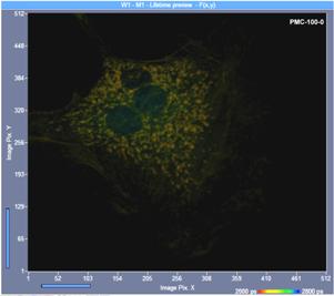
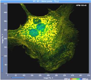
Fig. 14: FLIM image recorded with a conventional PMT (bh PMC-100-00, left)
and a hybrid PMT (bh HPM-100-40, right). Identical imaging conditions, same
acquisition time. The HPM-100-40 image contains 4.2 times more photons than the
image taken with the conventional PMT.
The SNR of the obtained lifetimes is
proportional to the number of photons per pixel. In principle, the SNR under
photon-limited conditions can therefore be increased by decreasing the number
of pixels. For example, a 128 x 128 pixel image needs only 1/16 of the
photons of a 512 x 512 pixel image. The flaw of this approach is that
it trades lifetime accuracy against spatial resolution. Unless there are other
arguments for low pixel number, such as data size or scan speed, it is
therefore not recommended to decrease the pixel number below 256 x 256.
A far better way is to record the images with a pixel number that yields
adequate spatial sampling, and use pixel binning in the data analysis [3], see
section 'Data Analysis' for details. Pixel binning in the data analysis leaves
the number of pixels unchanged, but runs the lifetime analysis on the sum of
the decay data of the current pixel and the pixels around it. The advantage is
that there is no loss in spatial resolution and no spatial undersampling, and
that you are free to select the best binning factor on the readily recorded
data. An example is shown in Fig. 15. The data in the top row were recorded in
a 128 x 128 pixels scan, the data in the bottom row by a
512 x 512 pixel scan. Both recordings contain the same total number
of photons. Consequently, the number of photons per pixel by the
512 x 512 pixel scan is 16 times lower. However, the lower photon
number was compensated by binning of pixels in the data analysis. The decay
curves per binning area (bottom row) therefore contain the same number of
photons as the decay curves per pixel (top row). Consequently, the lifetime
histograms (shown on the right) have the same width for both recordings.
However, the image from the 512 x 512 pixel scan (bottom row, left)
is much sharper than the one from the 128 x 128 pixel scan (top row,
left). Please see section 'Data Analysis'.
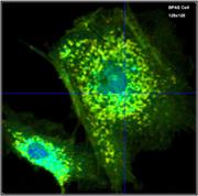
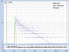
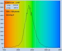

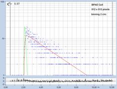
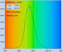
Fig. 15: FLIM data recorded with different pixel numbers. Same acquisition
time, same total number of photons. Upper row 128 x 128 pixels, lower
row 512 x 512 pixels. Left to right: Images, decay curves at cursor
position, lifetime histogram. The 512 x 512-pixel image was analysed with
pixel binning to compensate for the lower number of photons per pixel.
As described under 'Signal-to-Noise Ratio'
a TCSPC system is able to reach the theoretical signal-to-noise ratio given by
SNR = SQRT (N). This requires, however, that that every fluorescence photon
seen by the detector adds its maximum possible amount of information to the
result. This requires that the TCSPC timing parameters are correctly configured,
that the recording of background photons is avoided, and that the photon times
are determined at sufficiently high precision. These and a few other points
will be considered in this section.
The observation time interval (the time
interval over which the photon times are determined) can have an influence on
the signal-to-noise ratio of the lifetime. Fig. 16 shows an example. Two images
of the same sample were taken, with the same count rate and the same
acquisition time. The laser repetition rate was 50 MHz. The left image was
recorded within an observation-time interval of 5 ns. The lifetime is
about 2.2 ns. Therefore the fluorescence does not fully decay in the observation-time
interval, see Fig. 16, second row, left. As a result, photons in the tail of
the decay functions are not recorded, and the data analysis procedure can
determine the lifetime from the recorded part of the decay only. The
distribution of the lifetimes over the pixels is therefore broader than it
would be under ideal conditions, see Fig. 16, bottom left. The situation shown
in Fig. 16 is not unrealistic. Short observation time intervals can be fully
appropriate for samples with extremely short lifetime. It can then happen that
they are unintentionally used for long lifetimes as well, with the result that
a sub-optimal photon efficiency is obtained.
The image on the right was recorded within
an observation-time interval of 12 ns. Virtually all photons of the decay
function are recorded, and data analysis has the entire decay function to
determine the lifetime from, see second row of Fig. 16, right. As a result, the
distribution of the lifetime (Fig. 16, bottom right) is narrower than for the
5-ns recording.
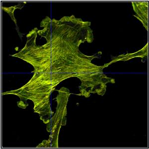
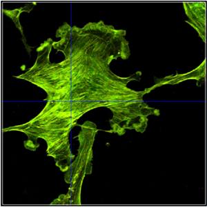
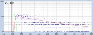
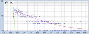
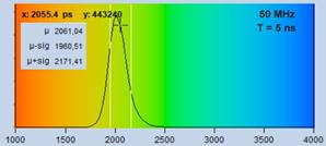
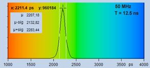
Fig. 16: Images recorded within an observation time interval of 5 ns
(left) and 12 ns (right). Decay curves and histograms shown in the second
and third row.
Also the way the decay curves are placed in
the observation time interval can have an influence on the photon efficiency. Fig.
17 shows an example. For the left image, the decay curves have been improperly
placed in the observation time window. The curves are shifted to the right, so
that the far end of the decay curve is not recorded. The mistake in the
parameter setup in Fig. 17, left, may look trivial and easy to correct [2].
Nevertheless, the situation is frequently encountered in TCSPC FLIM data.
In the right image, the decay data are
perfectly placed in the observation time window, and the entire decay curve is
recorded. Not only is there no loss of photons, a fit routine also has a larger
time interval over which it can determine the lifetime. Consequently the
lifetime histogram for the correctly centred decay data is visibly narrower,
see Fig. 17, bottom. The standard deviation, st, is 80 ps versus 118 ps for
the data on the left. This is a ratio of 1.48 in favour of the well centred
decay data. A ratio of 1.48 in st may not
sound very much. However, it translates into a factor of 2.18 in photon
efficiency. That means the correctly configured system needs 2.18 times less
photons (or 2.18 times less acquisition time!) to reach the same lifetime
accuracy as the system on the left.
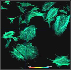
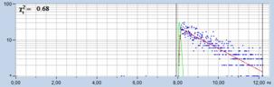
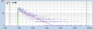
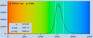
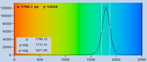
Fig. 17: Effect of sub-optimal recording of the decay curves. In the left
image, the decay curves are improperly placed in the observation time window.
The far end of the decay curve is not recorded. In the right image, the decay
data are perfectly placed in the observation time window. The entire decay curve
is recorded. The lifetime histogram for the correctly centred decay data is
noticeably narrower.
A comparison of the lifetime images in Fig.
16 and Fig. 17, left and right, shows also another effect: The lifetimes in the
left images are biased toward smaller values. The reason is that the
fluorescence decay is not purely single exponential. The slow decay component
is most prominent in the tail of the decay curve, i.e. in he missing part of
the data. When the data analysis procedure fits the data with a
single-exponential model it can optimise the fit for the recorded part of the
decay data only. In this part the slow component is under-represented, with the
result that the lifetime is determined shorter than it actually is. The
situation for the first-moment technique is even worse. Since the tail of the
fluorescence decay is missing the calculated moment is too small, and so is the
fluorescence lifetime derived from the first moment.
FLIM systems using ps diode lasers can be
operated at different laser repetition rates [5, 6, 7]. Standard rates are 20 MHz,
50 MHz, and 80 MHz, but other repetition rates can be built in on demand.
Multiphoton FLIM systems using Ti:Sa lasers are running at 80 MHz, and
systems with femtosecond fibre lasers often use 40 MHz [17]. Which
repetition rate is best? Can a fluorescence lifetime of 5 ns still be
accurately determined with 80 MHz repetition rate? Should I possibly always use
80 MHz because there is more excitation power available?
Fig. 18 shows decay curves from a selected
spot within the scan of a dye solution. The fluorescence lifetime is
5.6 ns. The upper curve was obtained with 50 MHz, the lower curve
with 80 MHz repetition rate. The number of photons is about 20,000 and
approximately the same in both curves. Both curves contain a substantial amount
of 'incomplete decay' from photons that remain from the previous excitation
pulse. The amount of incomplete decay is, of course, higher in the 80 MHz
recording because there is less time for the fluorescence to decay. For obvious
reasons, data with incomplete decay cannot be analysed by the first-moment
technique. They can, however, be processed with the 'incomplete decay' models
of SPCImage. Processing the images this way yields the lifetime distributions
shown in Fig. 18, right.
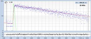
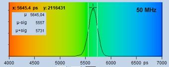
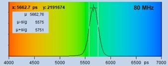
Fig. 18: Fluorescence decay functions from a dye solution, 5.6 ns
fluorescence lifetime. Top: Laser repetition rate 50 MHz. Bottom: Laser
repetition rate 90 MHz. Left: Decay curves. Right: Histograms of the
lifetime over the pixels.
The result is a surprise: Although the 50‑MHz
curve looks much more 'analysis friendly' the histograms are virtually
identical. Why? The reason is that the sum of a 5.6 ns decay and another 5.6‑ns
decay shifted by one period left is still a 5.6‑ns decay. The fit
procedure therefore delivers the correct lifetime with a reasonable standard
deviation. The standard deviation is larger that the ideal value for 20,000
photons but it is the same for both recordings. The loss against an ideal
recording comes from the fact that the recording time interval does not cover
the entire decay, not from the fact that incomplete decay is present. This is
supported by Fig. 19. It shows a recording at 50 MHz but within an observation-time-interval
of 20 ns. The lifetime distribution obtained from these data is noticeable
narrower.
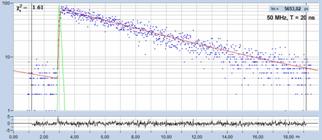
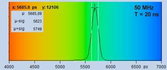
Fig. 19: Fluorescence decay of 5.6 ns, recorded with 50 MHz repetition
rate and within a recording time interval of 20 ns.
The conclusion is: If possible, use a
recording time window that covers as much as possible of the fluorescence
decay. If you can't do so because the laser pulse period is too short, don't
worry. Data analysis will takes care of the incomplete decay and extract the
best lifetime information possible.
Counting background is not only the most
common flaw in FLIM data, it is also the most devastating one. Fortunately, it
is also the one that is easiest to avoid. In most cases, the background just
comes from pickup of daylight. Most vulnerable are multiphoton systems with
non-descanned detection. These systems have no pinhole that rejects light from
outside the excited spot. They are designed to detect photons that are
scattered on the way out of the sample. To do so, they collect light from a
large area of the sample surface. The side effect is that they are also
sensitive to ambient light. Keeping off daylight from the detection system is
therefore imperative.
Fig. 20 shows what happens if the decay
data are overlaid by background counts. The fluorescence photons (a) have an
average arrival time <t> = t, and a timing noise of st = t. Could we build up a photon distribution of the fluorescence
photons alone, it would represent the true fluorescence decay curve (a, right),
an deliver the fluorescence lifetime with a standard deviation of st = t / SQRT (N),
i.e. with a photon efficiency of one.
The background photons (b) spread evenly
over the entire observation time window, T. Their average arrival time is T/2,
and their timing noise is stbkg= 0.28 T (see Fig. 24, page 25).
The recording process makes no difference
between fluorescence and background photons. The detected signal (c) is
therefore the sum of the fluorescence decay and the background. This causes two
unpleasant effects. First, the average arrival time is no longer the
fluorescence decay time, t. Instead, it is a photon-number weighted average of the lifetime, t, and the
average arrival time of the background photons, T/2. The data therefore cannot
be analysed by the first-moment technique, or by any other technique based on
moments.
Second, the effective timing noise is a weighted
sum of the timing noise of the fluorescence photons, st = t, and the timing noise of the background, stbkd = 0.28 T. In most instances 0.28 T is larger than t. It thus has a
large influence of the net standard deviation, stmeas of the
measured lifetime. An exact calculation of stmeas and thus of
the photon efficiency is difficult and delivers results which cannot easily be interpreted.
Nevertheless, the considerations above show that counting background has a
large effect on the detected lifetimes.
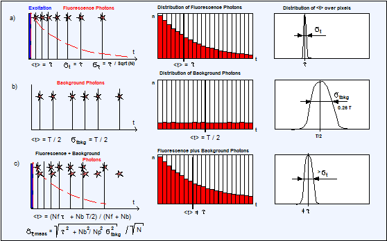
Fig. 20:
Effect of counting background on the photon times
A practical example is shown in Fig. 21. FLIM
images from the same sample were recorded with background (left) and without
(right). In the left image, the background in each pixel is about 900 counts
(sum over all time channels), in the right image it is close to zero. The
number of fluorescence photons in the brightest pixels is about 4000. The
background therefore visibly impairs the contrast of the image, see Fig. 21,
left. The loss in contrast is no so bad, however, to obscure the image entirely.
The right image is free of background and thus provides maximum contrast.
The decay curves in a selected spot are
shown in the second row. The decay curve from the left image contains
background counts, the decay curve from the right image does not. The
background seems moderate and does not look like a real problem. Nevertheless,
the effect on the lifetime accuracy is enormous. This can be seen in the third
row of Fig. 21. It shows, for each of the recordings, a phasor plot, and a
histogram of the lifetime calculated by first moments. It can easily be seen
that the histogram and the phasor plot for the left data set are not only
entirely off but also extremely widened. The reason is not only that the
background adds timing noise to the photon data but also that the background
adds an offset to the moments. Since the ratio of fluorescence and background changes
with the brightness of the pixels the lifetime values get extremely smeared
out.
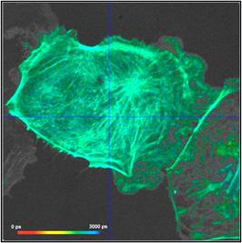
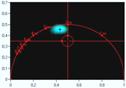
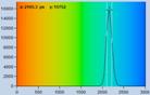
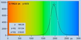
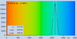
Fig. 21: Effect of counting background on FLIM accuracy. Left: FLIM data
with background counts. Right: Background-free recording. Upper row: Images.
Second row: Decay data in selected spot. Third row: Phasor plots and lifetime
histograms of M1 analysis. Lower row: Lifetime histograms from MLE analysis.
The bottom row of Fig. 21 shows histograms
of the lifetimes obtained by MLE analysis. In terms of lifetime shift the fit
procedure does better than moment analysis. Nevertheless, the lifetime is by
about 170 ps off, and the histogram is by a factor of two wider than that
of the background-free recording on the right. A factor of two in lifetime standard
deviation translates into a factor of four in photon efficiency!
In contrast to widespread opinion, the
number of time channels in the decay curves has no direct influence on the
signal-to-noise ratio. It does not appear in the equation of the SNR (section 'Signal-to-Noise
Ratio') derived for first-moment analysis, and data analysis by fit routines does
not care whether FLIM data have half the number of photons in twice the number
of time channels or vice versa. Only the total number of photons in the decay
curve matters. An experimental verification is given in Fig. 22. It shows a
sample stained with Alexa 488. At the detection wavelength used, the lifetime
is almost uniform over the entire scan area. The data in the first row were
recorded with 64 time channels, the data in the second row with 1024. The total
number of photons in the images is virtually the same. As expected, the lifetime
histograms (first and second row, right) are almost identical.
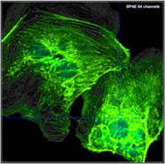
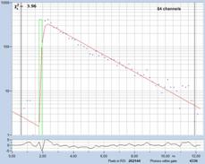
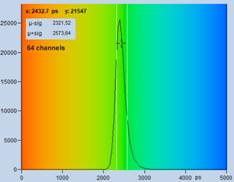
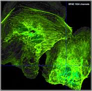
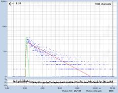
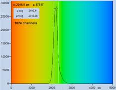
Fig. 22: Recording with different number of time channels, same total number
of photons. Upper row: 64 time channels. Lower row: 1024 time channels. Left to
right: Image, decay curve at cursor position with single-exponential fit, histogram
of lifetime over the pixels. In contrary to widespread opinion the higher
number of photons per time channel in the 64-channel recording does not yield
to a higher lifetime accuracy.
The fact that the SNR of the lifetime is
independent of the number of time channels does not mean that arbitrary small
numbers of time channels and arbitrary large time-channel widths can be used. Detecting
in just two or four time channels massively decreases the photon efficiency [1, 13, 19]. However, degradation of the SNR
already starts when the time channel width is on the order of the IRF width. It
is then not clear where in the first time channel the IRF is located, and where
the rise of the fluorescence pulse starts. This adds uncertainty to the
lifetime determination. As a rule of thumb, both the IRF and the fastest decay
component should be sampled with no less than 5 to 10 time channels. That means,
for an HPM-100-40 detector (IRF width 120 ps) and fast decay components
down to 100 ps the time channel width should be about 10 ps. For an
observation-time interval of 10 ns the number of time channels should then
be 1024. For an HPM-100-06 (IRF width <20 ps) it is not ridiculous to
increase the number of time channels to 4096, i.e. decrease the time channel
width to 3 ps. Even narrower time channels may be appropriate if
ultra-fast decay components are to be detected.
What happens if the IRF of the FLIM system
has non-zero width? The effect of the IRF can, again, be estimated by looking
at the photon arrival times. Let's assume that we have recorded or otherwise
determined the IRF of the FLIM system. We can then define a 'centroid' of the
IRF by averaging the photon times from the IRF measurement, <tirf>.
As shown already in Fig. 6, page 9, the fluorescence decay time, t, is obtained by
simply subtracting <tirf> from the average photon times
<t>, see Fig. 23, left.
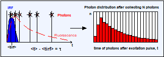

Fig. 23: Standard deviation of lifetime measurement in a system with
no-zero IRF width. Left: The lifetime is the average arrival time, t, of the
photons minus the time of the IRF centroid, <tirf>. Right: The
standard deviation of the measured lifetime, tmeas, contains a contribution from the IRF, sirf.
What is the standard deviation of the
lifetime obtained this way? One could presume that the standard deviation is
still t / SQRT(N): The centroid of the IRF is accurately known,
and subtracting it does not change the standard deviation of t. This is wrong.
It is wrong because the photon times themselves now contain an uncertainty from
the IRF. Every fluorescence photon has its timing reference at a different time
in the IRF. It may have been excited at a different time in the laser pulse, or
it has spent a different time transiting the detector. This adds an uncertainty
to the photon times, t, and adds a contribution of the IRF, sirf , to the standard deviation, st = t, of the ideal photon times.
The standard deviation of the measured photon
times stmeas is therefore larger than t, and the
standard deviation of the measured lifetime, stmeas , is
larger than t / SQRT(N). It can be estimated by quadratically adding the standard
deviation of the photons in the ideal fluorescence decay, t, and the
uncertainty from the IRF, sirf :
stmeas = SQRT (t2 + s2irf) / SQRT (N) or
1
SNRtmeas = SQRT (N) × SQRT ------ )
(1
+ s2irf / t2)
sirf is also known as 'RMS Timing
Jitter' or - a bit misleading - 'IRF width RMS'. For IRF shapes
encountered in practice it is about 0.43 to 0.87 of the full-width at half maximum
(FWHM) of the IRF. The RMS versus the FWHM values for a few typical IRF shapes
are given in Fig. 24. For a Gaussian IRF the RMS timing jitter is
0.43 FWHM. For asymmetrical functions it is larger than this. IRFs with
slow tails or with bumps add more timing noise to the decay data, and should,
if possible, be avoided. Please note that tails and bumps can also originate
from picosecond diode lasers operated at excessively high power. The accuracy
loss by the unfavourable IRF shape can in fact outweigh the gain from the
increased number of photons.
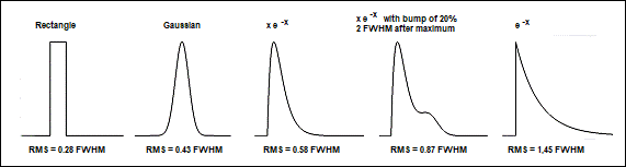
Fig. 24: RMS values for a number of
typical IRF shapes. Left to right: Rectangle, Gaussian, x×e-x,
x×e-x
with a bump 2 FWHM after the maximum, exponential function e-x.
Functions normalised to same FWHM, RMS values given in fractions of the FWHM.
There are two conclusions from this result.
The first one is that, not surprisingly, the SNR still scales with the square
root of N. The second one is that a massive decrease in SNR occurs only when
the RMS of the IRF width becomes larger than about 50 to 100% of the
fluorescence lifetime.
The slow degradation of the lifetime
accuracy with increasing IRF width is surprising. It has led to the misconception
that the IRF width of a FLIM system is not important: The fluorescence
lifetimes of typical fluorophores are in the range of a few nanoseconds.
Therefore an IRF width of 500 ps to 1 ns (RMS) should be sufficient,
if only the IRF is exactly known. However, this contradicts any practical experience.
Where is the mistake?
The fluorescence decay functions in FLIM
are not single-exponential. More than that, the desired information often is in
the composition of the decay function rather than in the net 'lifetime'. In
that case, the IRF must be faster than the fastest decay component. Major decay
components in FRET measurements and in autofluorescence measurements range down
to about 300 ps and 100 ps, respectively [2]. The HPM-100-40 detector is a good match
to these applications. Lifetimes down to the 10 ps range are encountered
in mushroom spores [15], in human hair, and in lesions of mammalian skin. These
measurements require an even faster detector. Examples will be shown in section
'Multi-Exponential Decay Functions'.
A single-exponential approximation of the
fluorescence decay and the measurement of its apparent lifetime may be
sufficient when FLIM is just used as a contrast technique in laser scanning
microscopy. However, the real applications of FLIM are in molecular imaging.
Fluorophores - either endogenous or exogenous ones - change their fluorescence
lifetimes depending on their molecular environment. This may be binding to
proteins, protein configuration, interaction of proteins with others, effects
of the metabolic state of cells or tissues, or the concentration of ions
involved in the function of the cells. In these applications the task is not to
distinguish different fluorophores but to distinguish fractions of the same
fluorophore in different molecular environment and quantify them by their
relative concentrations [1, 4, 18]. In most cases this requires recording of
multi-exponential decay functions and splitting them into different decay
components. Multi-exponential decay recording and multi-exponential decay analysis
are therefore standard in FLIM of biological systems. A few examples are shown
in Fig. 25 and Fig. 26. More examples of multi-exponential FLIM measurements
are shown in Fig. 31, Fig. 32, and Fig. 41.
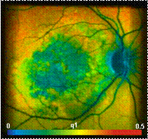
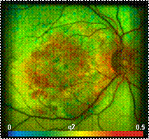
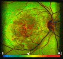
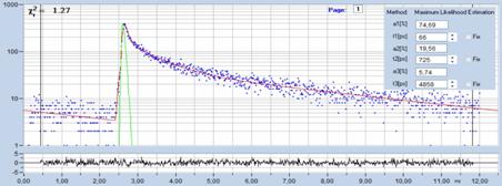
Fig. 25: Top: FLIM Images of the human retina, recorded in vivo. Intensity
contribution of the fast, medium, and slow decay component. Bottom: Decay curve
in selected spot of the image. Data courtesy of Dietrich Schweitzer and Martin
Hammer, University of Jena.
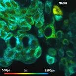
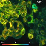
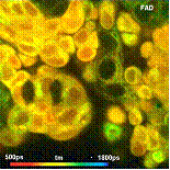
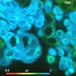
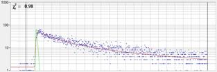
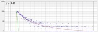
Fig. 26: Metabolic imaging by FLIM of NADH (left) and FAD (right). Images
of the amplitude-weighted lifetime, tm, of double-exponential decay, and of the
amplitude of the fast decay component, a1. Bottom: Decay functions in selected
spot of the NADH and the FAD image.
Extracting individual decay components from
a multi-exponential decay analysis requires more photons than a single-exponential
fit or first-moment analysis [20]. Therefore, detection efficiency and photon
efficiency are the crucial parameters. Time resolution is important as well -
the requirements to the IRF width are given by the lifetime of the fastest
decay component, not by the apparent lifetime of the net decay function.
What also matters is the shape of the decay
functions. The more they differ from a single-exponential decay the better. Decay
components that have nearly the same lifetime are hard or impossible to split [20],
and decay components with low amplitudes are difficult to extract. Three
examples are shown in Fig. 27. The function shown left contains 82 % of
445 ns on the background of 2.4 ns. It is easy to resolve. The
function in the middle is more difficult. The amplitude of the fast component
is only 24 %, and the lifetime is almost 900 ps, compared to
2.5 ns of the slow one. The net decay function is much closer to single-exponential
than the one on the left. The decay profile on the right is visually
indistinguishable from a single-exponential decay. It contains 35 % of
3 ns and 65 % of 4.5 ns. With the number of photons typically
available in FLIM it cannot be resolved on a pixel-by-pixel basis.
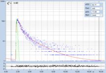
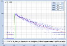
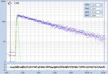
Fig. 27: Double-exponential decay functions. The function on the left is
easy to resolve, the function in the middle is difficult, and the one on the
right is virtually impossible to resolve in FLIM data.
Situations as the one shown in Fig. 27,
right, should, if possible, be avoided already in the experiment planning. An
example are FRET experiments: FRET pairs with large donor-acceptor overlap and FRET
constructs with short donor-acceptor distance and large fractions of
interacting donor deliver donor decay functions with a large amplitude and a
short lifetime of the fast component. This make it easier to resolve the decay
profile, and thus separate interacting and non-interacting donor fractions.
In some cases the results can be massively
improved if the signals are spectrally separated. The number of decay
components is then reduced, and the analysis becomes easier. Spectral
separation can be obtained both on the excitation and on the detection side. An
example is metabolic imaging by NADH / FAD FLIM. When both
fluorophores are excited at the same wavelength (as it is often attempted) and only
observed through different emission filters the situation can be virtually hopeless.
However, by multiplexed excitation and detection in the right wavelength
intervals the signals can be well separated [18]. Experiment planning, both in
terms of sample design and FLIM configuration, therefore has a large influence
on the quality of the results.
Fig. 28 and Fig. 29 give examples of
multi-exponential decay measurement. Fig. 28 shows FLIM data of an NADH
solution. A solution was used to obtain a homogeneous lifetime distribution
over the entire scan area. The parameter histograms over the pixels are then
determined by the photon noise, not by lifetime variation over the scan area.
The data were recorded with two-photon excitation at 785 nm, images were
scanned with 512 x 512 pixels, 1024 time channels. From top to
bottom, Fig. 28 shows data recorded with a H7422-40 PMT detector, and by
HPM-100-40 and HPM-100-06 hybrid detectors. The IRF widths are 250 ps,
110 ps, and 18 ps, respectively. From left to right, the figure shows
a decay curve in an arbitrary selected spot, a histogram of the lifetime of the
fast component, t1, a histogram of the second fast component, t2, and a
histogram of the slow component, t3.
It can clearly be seen that the lifetime
histograms become narrower with decreasing IRF width. Interestingly, this is
not only the case for the fast component but also for the medium and slow
component. The best result is obtained with the HPM-100-06, i.e. with an IRF
width of 18 ps. Decay data recorded with an IRF this fast are virtually unimpaired
by IRF-induced timing jitter. The histograms of t1, t2, and t3 are by a factor
of 1.4 narrower than for the H7422. That means the photon efficiency for the
fast detector is 2 times higher.
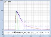
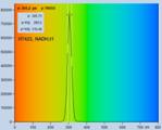
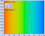
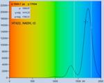
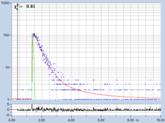
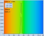
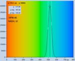
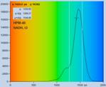
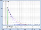
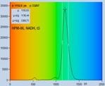
Fig. 28: NADH solution, data recorded with different detectors. Upper row:
H7422-40 detector, IRF width 250 ps. Second row: HPM-100-40, IRF width
110 ps. Lower row: HPM-100-06, IRF width 18 ps. Left to right: Decay
curve in arbitrary selected spot, histogram of the fast component, t1,
histogram of the second fast component, t2, histogram of the slow component,
t3. Two photon excitation, non-descanned detection, images 512 x512 pixels,
1024 time channels, about 5000 photons in binning area.
Fig. 29 gives an example of the detection
of an ultra-fast decay component with sub-25ps lifetime. Such fast components
are more frequent than commonly believed. We find them routinely in human hair,
mushroom spores and in nevi of mammalian skin. A fast component exists also in the
fluorescence decay of Flavine Adenine Dinucleotide, FAD, a natural fluorophore
that is present in every cell. FAD is important because its fluorescence decay function
contains information on the metabolic state of the cell.
Fig. 29 shows FLIM images of an FAD
solution. Left to right, the figure shows images of the fast decay component,
t1, of a triple-exponential fit, a decay curve, and a histogram of t1. The data
in the upper row were recorded with an HPM-100-40 detector, the data in the
lower row with an HPM-100-06. Visually, the decay curve recorded with the
HPM-100-40 (IRF 110 ps FWHM) shows no trace of a fast component. However, careful
data analysis extracts a component with a lifetime on the order of 20 ps. It
would elude attention unless it is explicitly searched for. The histogram of
the t1 values over the entire image is shown on the right.
The lower row of Fig. 29 shows data
recorded with an HPM-100-06 (IRF width 18 ps FWHM). The decay curve convincingly
shows that the fast component is indeed present. Data analysis in the selected
spot of the image delivers a lifetime, t1, of 16.5 ps for the fastest
component (the other two components are 2.2 ns and 3.2 ns). The histogram
shows that the most frequent t1 value is about 16 ps. As expected from the
fast IRF, the histogram is by almost a factor of 2 narrower than that for the
HPM‑100‑40 data.
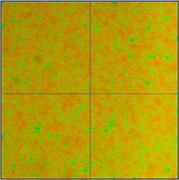
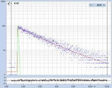
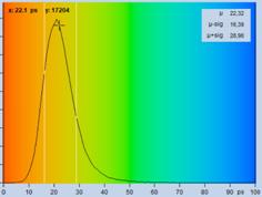
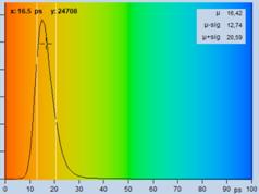
Fig. 29: Fluorescence of an FAD solution. Left to right: Image of the fast
decay component, t1, of triple-exponential analysis, decay curve, histogram of
t1. Upper row: Recorded with HPM-100-40 detector, IRF width 110 ps FWHM.
Lower row: Detected with HPM-100-06, IRF width 18 ps FWHM.
It should be noted that there is a
potential conflict between the IRF width and the efficiency of the detector.
The fast detectors have conventional bialkali photocathodes. They are thus
about 4 times less sensitive than the GaAsP detectors. It is not a priori clear
whether faster IRF or higher sensitivity is more important. Certainly, for
resolving ultra-fast decay components there is no way around the fast IRF. It
is a big difference whether you actually see the fast component or have
to squeeze it out from the data by deconvolution. We also found that double-
and triple-exponential decay analysis of NADH and FAD data is more reliable
with a sub-20-ps IRF [2, 16].
This can also be seen in Fig. 28, bottom. In practice the decision for one
detector or the other depends on the photostability of the sample. If the
sample remains stable under four times the excitation power or during four
times the acquisition time the fast detector is the right one. If it doesn't
the GaAsP detector must be used.
The FLIM literature is full of incorrect
statements on the 'Pile-Up' effect and its influence of FLIM results. Pile-Up
is the detection of a second photon in the same laser pulse period with a the
first one. As a result, the second photon is lost, and the recorded decay
profile gets distorted. Truth is, that the influence of pile-up on FLIM
results is vastly over-estimated. A mathematical analysis of the pile-up effect
is described in [1] and [2]. It
turns out that FLIM can be recorded at count rates up to 10% of the laser pulse
repetition rate without noticeable error in the recorded decay data. For
typical pulse repetition rates of 50 to 80 MHz this is higher than a
typical FLIM sample can deliver.
Pile-up should not be confused with 'Counting
Loss'. Counting loss is the loss of photons within the dead time (the signal
processing time) of the TCSPC module after the detection of a previous photon.
Counting loss has no immediate influence on the decay data but has an influence
on the recorded intensities. With increasing count rate the intensity
characteristics becomes nonlinear, flattens and, finally, saturates. As a
result, the images are losing contrast an get an ugly 'flat' appearance. For
the SPC-series FLIM modules this becomes noticeable at detector (CFD) count rates
of 5 to 10 MHz.
The effect of counting loss can be avoided
by the 'Lifetime-Intensity' mode of the bh TCSPC FLIM modules [10]. The mode is
using a fast counter in parallel with the TCSPC timing electronics. The SPCM
data acquisition software builds up FLIM images by using pixel intensities from
the parallel counter and pixel decay data from the timing electronics. A
comparison is shown in Fig. 30. If you see a loss in contrast as in Fig. 30,
left, pass to the INT-FLIM mode. Details are described in [10].
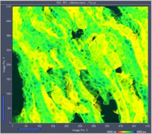
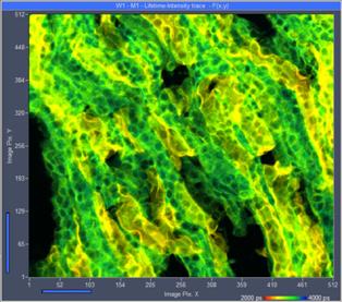
Fig. 30: High-count rate images recorded from an Invitrogen F24630 Mouse
kidney section. Left: Traditional FLIM mode. Right: Lifetime/Intensity mode.
Average (recorded) count rate 5.5 MHz.
Data analysis cannot compensate for poor
quality of FLIM data if these have been carelessly recorded. However, FLIM data
analysis can extract a wealth of information from data which have been recorded
from optimally designed samples and with the necessary care [3]. The section below addresses just a few
important points and demonstrates them on typical FLIM data.
The first question when it comes to FLIM
data analysis is usually: Which model do I have to use? How many exponential
components are necessary to fit the results?
The answer does not depend on the number of
decay components the sample actually has. It rather depends on what you want to
find out from this sample. Therefore, no one except yourself can answer the
question. You have a hypothesis of what is going on in a specific biological
system. You design an experiment and a sample to confirm or exclude the
hypothesis. Only you can know what is expected to happen in your sample, and
only you can know how many components are to be expected in the decay
functions. Therefore, you should select different models and make sure that the
model (and only the model) with the corresponding number of decay components
fits the data.
Here is an example. You are doing a
protein-interaction experiment. You are using FRET as an indicator of protein interaction.
You label one protein with a donor, the other with an acceptor. In places where
the proteins interact FRET should occur. FRET reduces the lifetime of the
donor. You therefore acquire FLIM data at the donor emission wavelength.
You load the data in SPCImage and run the
analysis with a single-exponential model. The fluorescence lifetime is shortest
in the cell membrane - exactly where you expect the proteins to interact (Fig. 31,
left).
You check the decay functions in a few
characteristic spots of the image. In places where the lifetime is short a single-exponential
model does not fit the decay functions properly, but a double-exponential one
does (Fig. 31, second left). This is plausible: First, not all donor molecules
have the right orientation to an acceptor for FRET to occur. Second, protein
interaction is a chemical equilibrium, and there should be a mixture of
interacting and non-interacting donor. These fractions have different lifetime,
consequently the decay profile should be double-exponential.
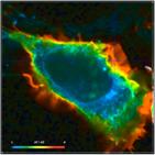
Fig. 31: Results of a FLIM-FRET measurement. Left to right:
Single-exponential lifetime image, decay curve at cursor position, image of
amplitude-weighted lifetime of double-exponential model, showing classic FRET
intensity, image of amplitude ratio, showing relative fraction of interacting
proteins.
Now you run data analysis with a
double-exponential model. For display, you select the amplitude-weighted mean lifetime,
tm. This is the representation of the classic FRET efficiency. The image is
shown in Fig. 31, second right. Next, you select the ratio of the amplitude of
the fast and the slow decay component. The ratio indicates the relative amounts
of interacting and non-interacting donor. It is highest in the cell membrane,
where you expect the proteins to interact, see Fig. 31, right. The result shows
that a double-exponential model is appropriate to fit the data, and it shows
that the initial hypothesis is likely to be correct.
SPCImage offers several options to display
parameters of the decay functions. Available are the classic single-exponential
lifetime, lifetimes of decay components, the amplitude-weighted average and the
intensity-weighted average of the component lifetimes, and relative intensities
contained in the decay components [3]. SPCImage also displays ratios of these
parameters. If possible, a parameter combination should be selected that shows
the effect of interest most clearly. For example, in a FRET measurement the
amplitude-weighted lifetime of a double-exponential fit, represents the classic
FRET efficiency, and the ratio of the amplitudes, a1/a2, the relative fraction
of interacting donor. Examples are shown above in Fig. 31.
An examples for metabolic imaging is shown
in Fig. 32. The image on the left shows the amplitude ratio of the decay
components from free and bound NADH. This parameter characterises the metabolic
state of the cells. The images of the component lifetimes, t1 and t2, are shown
middle and right. The inhomogeneity of the lifetimes indicates different
molecular environment of the NADH in the individual mitochondria.
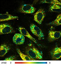
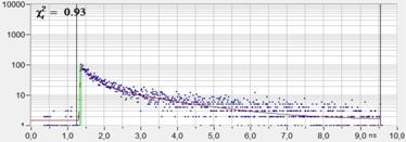
Fig. 32: Left to right: NADH images of live cells. Images of the amplitude
ratio, a1/a2 (unbound/bound ratio), and of the fast (t1, unbound NADH) and the
slow decay component (t2, bound NADH). FLIM data format 512x512 pixels. Bottom:
Decay curve in selected spot. 1024 time channels. time-channel width 10ps.
Binning of lifetime data is often
disapproved of by FLIM users as a way of unscientifically tweaking measurement
results. However, correct binning is key to any accurate and reliable FLIM data
analysis.
When an image is recorded by an optical
system the spatial resolution is limited by diffraction. The diffraction
pattern for a single point of light is called Airy disc or (in microscopy)
point-spread function. To reach diffraction-limited resolution the data must
not be blurred additionally by pixelling. As a rule of thumb, the central disc
of the point-spread function should be sampled by about 5 x 5 pixels.
Of course, the lifetime information in the pixels within this area is closely
the same. It is therefore appropriate to combine the temporal data of these
pixels for FLIM analysis, see Fig. 33, left. The result is a substantial
increase in the photon number and a corresponding increase in lifetime
accuracy. Please note that combining a 5 x 5 pixel area increases of
the net photon number by a factor of 25!
In SPCImage binning is performed by
combining the data from a defined binning area and assigning the net decay
curve to the central pixel. The effective number of pixels in the image is
therefore not changed. The procedure also meets an esthetical aspect of a good
image. Visually, an image can contain a large amount of intensity noise before
it starts to look ugly. The same amount of noise in the lifetime data would, however,
render the data useless for any kind of serious FLIM application. It therefore
makes sense to display an image at a large number of pixels with some intensity
noise, but with the lifetime averaged within larger areas and correspondingly
increased signal-to-noise ratio. The principle of binning in SPCImage is
illustrated in Fig. 33, right.
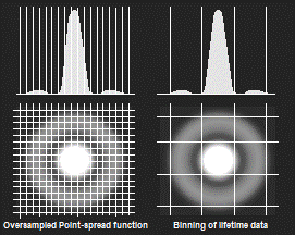
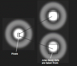
Fig. 33: Left: Oversampling of the Airy disc in the intensity image and
binned pixels for lifetime calculation. Right: Overlapping binning of pixels
for lifetime calculation.
The meaning of the binning parameter, n, in
SPCImage is illustrated in Fig. 34. Please note that a binning factor of two
corresponds to a 5 x 5 pixel area, i.e. roughly to the area of the
point-spread function in a correctly sampled image. Unintentionally, images are
often taken with higher oversampling, especially when high zoom factors of the
scanner are used. Therefore SPCImage provides binning factors of up to 10,
corresponding to an area of 20 x 20 pixels.
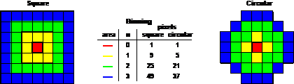
Fig. 34: Function of the binning parameter, n. Binning 'Square' (left) and
'Circular' (right).
A demonstration of the effect of binning is
given in Fig. 35. A BPEA sample was scanned with 512 x 512 pixels,
the decay curves were recorded into 1024 time channels. Data without binning
are shown in the top row of Fig. 35. A (single-exponential) lifetime image is
shown on the left. Without binning the number of photons per pixel is ridiculously
low, see second left. Consequently, the lifetime image looks noisy, and the
decay times scatter all over the place, see lifetime histogram on the right.
The bottom row of Fig. 35 shows data analysed with binning. A binning factor of
2 with circular binning was used, corresponding to a binning area of 21 pixels.
The lifetime image is of excellent quality, the net decay functions have enough
photons for a reasonable fit, and the lifetime histogram has a reasonable
width. As can be seen in the image, the colour does not blur out, i.e. binning
did not cause noticeable loss in the spatial resolution of the lifetime.
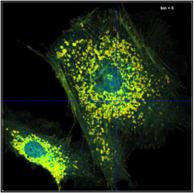
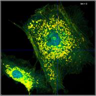
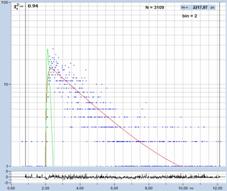
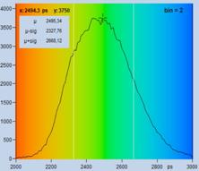
Fig. 35: Effect of binning in lifetime analysis. 512 x 512 pixels, 1024
time channels. Top: No binning. Bottom: Binning factor 2, circular binning. Sum
of decay curves of 21 pixel area is used for analysis of central pixel.
With a binning factor of 2 (decay curves
from 21 pixels binned into centre pixel, see Fig. 34) the data are even good
enough for double-exponential decay analysis. The result is shown in Fig. 36.
The top row, left to right, shows lifetime images of the fast decay component
and of the slow decay component, and an image of the ratio of the amplitudes of
the two components. All three images are of good quality, both in terms of
spatial resolution and lifetime resolution. The bottom row shows the parameter
histograms. They show that the component lifetimes and the amplitude ratio are
obtained at a good signal-to-noise ratio (please note the different parameter
ranges).
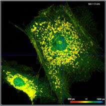
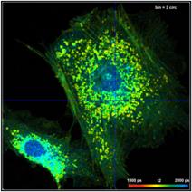
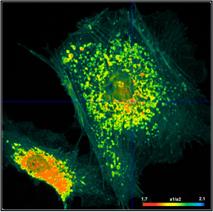
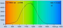
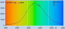
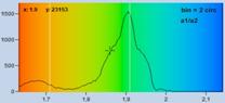
Fig. 36: Same data as in Fig. 35, bottom. Double-exponential decay
analysis. Left to right: Lifetime image of fast component, t1, lifetime image
of slow component, t2, image of amplitude ratio, a1/a2. Please note different
parameter ranges.
Fig. 37 shows the effect of binning on the
spatial resolution of the lifetime information. The figure shows data from a
70 x 70 pixel area in the centre of the large cell in Fig. 35 and Fig.
36. As expected, lifetime contrast remains largely unchanged up to binning = 2,
see the flower-like structure in the centre. For binning factors of 4 and 6
(second right and right) the lifetime contrast starts to degrade. Too many
decay data from adjacent pixels are mixed into the net decay functions. The
structure in the middle therefore more and more assumes the lifetime of its
closer environment.
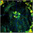
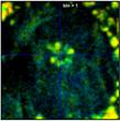
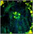
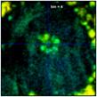
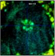
Fig. 37: Zoom into a 70 x 70 pixel area of the data of Fig. 35,
showing the centre of the large cell. Different binning, left to right bin = 0,
1, 2, 4, and 6. Lifetime contrast remains unchanged up to bin = 2
(centre image). It degrades at bin = 4 and bin = 6, as can be seen by a fading of
the colour of the structure in the centre.
In contrast to binning, which combines
spatially related pixels, image segmentation combines pixels which have a
similar decay signature.
The procedure is shown in Fig. 38. Upper
left, Fig. 38 shows the SPCImage panel with FLIM data of low photon number. The
data are the same as in Fig. 35, upper row. Decay data in a selected pixel are
shown in the lower right of the panel. The lifetime image calculated from these
data is noisy, and the histogram of the lifetime (upper right) is extremely
wide. The next step is shown in Fig. 38, upper right. A phasor plot is
calculated from the data. As expected, the phasors scatter all over the place.
Nevertheless, phasors from pixels with distinctly different lifetime (indicated
by colour) appear in different phase/amplitude locations.
In a third step, a range of phasor values
is selected, and the corresponding pixels are highlighted in the lifetime
image, see Fig. 38, bottom left. The selection area can be shifted and changed
in size and shape to highlight the desired structures in the image. In the
example shown, the mitochondria of the cell have been selected. Even though the
selection may be incomplete the selected pixels are all within the desired
structures of the image.
In the final step, Fig. 38, bottom right,
the decay data of the selected pixels are combined into a single decay curve.
This curve contains more than 3 million photons, compared to a few 100 in the
individual pixels, and to about 3000 in a binning area of two, compare Fig. 35.
A decay curve with 3 million photons can be analysed at high precision.
Triple-exponential analysis is no problem, as can be seen in Fig. 38, bottom
right. Triple-exponential decay parameters are displayed in the upper right
part of the panel.
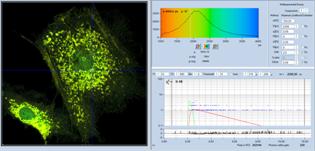
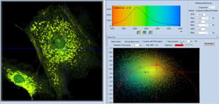
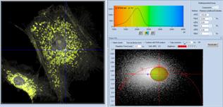
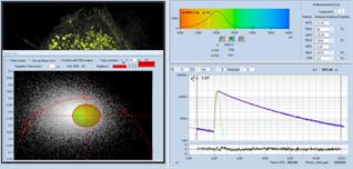
Fig. 38: Image segmentation via the phasor plot, and combination of the
selected pixel into a single decay curve of high photon number.
Motion in the objects to be imaged is a
general problem of laser scanning microscopy. It is an even bigger problem for
FLIM because it makes it impossible to collect a sufficiently large number of
photons for accurate FLIM analyis. As an example, Fig. 39 shows a leg of a live
waterflee. The leg is moving quickly so that even single 0.5 s frames
become badly distorted. The number of photons obtained within the 0.5 s frames allows
for approximate lifetime determination (see Fig. 39, right) but is insufficient
for precision decay analysis.
The solution is 'Temporal Mosaic FLIM' with
image segmentation [9]. A series of fast scans is recorded by the Mosaic
Imaging function of SPCM. The entire mosaic is loaded into SPCImage. A
preliminary data analysis is performed, and the result is loaded into the
Phasor Plot. In the phasor plot, a range with the decay signature of the leg is
selected. The decay data of all pixels of the selected signature are combined
into a single decay curve. This curve contains about five million photons and
can be analysed at high precision. Please see Fig. 40. The decay parameters are
shown upper right. The parameters of the first tow decay components are characteristic
of FAD, the third component even shows a trace of FNM [8].
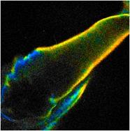
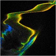
Fig. 39: Left
and middle: Moving leg of a live waterflee, 0.5-s scans. Right: decay curve in
a spot of 5x5 pixels.
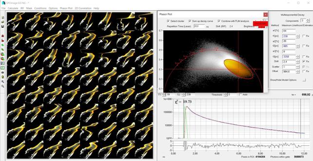
Fig. 40:
Left: Temporal Mosaic of the waterflee, 0.5 s per element. Right: Phasor plot.
Decay signature of the waterflee leg selected, decay data combined in a single
decay curve.
Multiexponential decay analysis becomes
easier if the number of decay parameters is reduced. Including a priori
knowledge in the data analysis can therefore reduce the noise in the results. Fig.
41 shows an NADH image of an open tumor in a mouse, imaged with the bh DCS-120
MACRO system. The interesting parameter is the amplitude, a1, of the fast decay
component. It represents the fraction of free NADH, and indicates the type of
the metabolism in the corresponding area of the tissue. The data were therefore
analysed with a double-exponential model, and a1 images were created. The image
on the left was analysed with all parameters, t1, t2, a1, a2, freely floating.
The image on the right was analysed with fixed t2. As expected, the image on
the right is less noisy. The tumor stands out more clearly, both in the image
and in the a1 histograms. The histogram on the right even displays two distinct
populations of pixels, one with a1 = 0.65 and one with a1 =
0.83. These are exactly the amplitudes typically found in healthy tissue and in
tumor tissue.
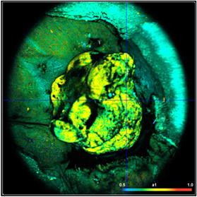
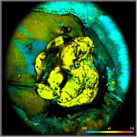
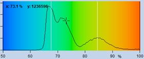
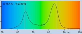
Fig. 41: NADH images of a mouse tumor showing the amplitude, a1, of the
fast NADH component. Left: T1, t2, a1, a2 floating. Right: t2 fixed to most
frequent value, 2400 ps. Lower row. Histograms of a1 over the pixels of
the image.
Analysis with fixed parameters can substantially
reduce the noise in cases where lifetimes of decay components are expected to
be constant. However, the technique has to be used with caution. Fluorescence
lifetimes are never absolutely constant. There is always an influence of the
molecular environment. If a component lifetime is fixed but not absolutely
constant the fit procedure responds with large changes in other parameters.
Therefore, fit results obtained with fixed component lifetimes can have large
systematic errors.
A FLIM image should clearly and plainly demonstrate
the scientific facts claimed in the associated publication. The images should
not only display the right decay parameters but also display them within an
appropriate intensity and decay-parameter range. As a default, SPCImage uses
autoscaling of the intensity. Under normal circumstances, autoscaling yields reasonable
images. However, the autoscale function cannot know which part of the image is
the one that contains the information of interest. If the information is in the
dim areas of the image autoscaling does not necessarily deliver the best
possible image. Also, it can happen that an otherwise perfect image contains a
few extremely bright spots. Wherever they come from, autoscaling does not yield
a reasonably scaled image in these cases. Autoscaling should therefore be
turned off and the intensity scale be adjusted manually. An example is shown in
Fig. 42. Autoscaling (left) leads to an unfavourably scaled intensity range. Manual
adjustment of the intensity range leads to a correctly balanced image (right).
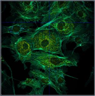
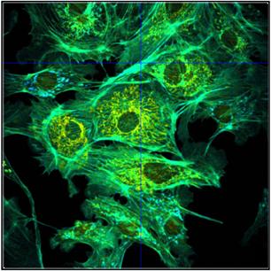
Fig. 42: Image containing a few extremely bright spots. Left: Autoscaling
of the intensity range. The autoscaling function scales the intensity to the
brightest features. The intensity range obtained is not appropriate for the
rest of the image. Right: Manual scaling yields an image within the right
intensity range. Lifetime of single-exponential fit, colour range from
2000 ps (blue) to 3000 ps (red)
The display of images with different
parameter scale is shown in Fig. 43 and Fig. 44. The figures show lifetime
images displayed with a colour direction blue-green-red and red-green-blue,
respectively. The parameter ranges are 2000 to 3000 ps (left) and 2300 to 2700
ps (right). Which style displays the effect of interest best must be decided
from case to case.

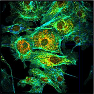
Fig. 43: Different representations of the data shown in Fig. 42.
Single-exponential lifetime, manual intensity scaling, colour direction b-g-r.
Left: Lifetime range 2000 to 3000 ps. Right: Lifetime range 2300 to
2700 ps.
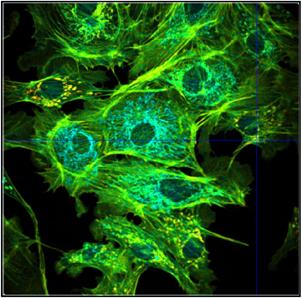
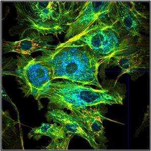
Fig. 44: Different representations of the data shown in Fig. 42. Single-exponential
lifetime, manual intensity scaling, colour direction r-g-b. Left: Lifetime
range 2000 to 3000 ps. Right: Lifetime range 2300 to 2700 ps.
The fluorescence lifetime can be derived
from TCSPC FLIM data at a signal-to-noise ratio close to square root of the
photon number per pixel. Therefore, the most important parameter that
characterises FLIM data quality is photon number. By using practical examples,
we have shown that by simply optimising the detection efficiency and the acquisition
time a factor of 10 in photon number can be gained. By using high-efficiency
detectors another factor of 4 can be added, and optimised binning strategies
can add a factor of 25. Altogether, this is a factor of 1000 in photon number,
or a factor of 32 in signal-to-noise ratio. We do not claim that an improvement
this large can be reached in all cases, but a sizable improvement is achievable
almost anytime.
The second important parameter of a FLIM
system is photon efficiency. Photon efficiency describes how efficiently the
individual photons detected by the system contribute to the result. In other
words, it describes how close the system gets to the ideal signal-to-noise
ratio, SQRT(N). Although TCSPC systems come close to the ideal, the photon
efficiency can often be optimised by using the correct TCSPC timing parameters,
by avoiding the recording of background signals, and by using sufficiently fast
detectors. Often an increase by a factor of two to four in photon efficiency is
possible by just obeying to a few simple rules of signal recording.
Data quality becomes especially important
when multi-exponential decay functions are recorded and analysed. In the most
frequent FLIM applications multi-exponential decays are rather the rule than
the exception. The information is then primarily in the amplitudes and
lifetimes of the decay components rather than in the apparent lifetime of the net
decay functions. That means not only detection efficiency and photon efficiency
are important but also the width of the instrument-response function. Moreover,
the options of resolving multi-exponential decay functions dramatically depend
of the shape of the decay functions. The more they deviate from a single
exponential profile the better they can be resolved. Therefore, experiment
planning and sample design with the options of FLIM in mind can have a massive
influence on the outcome of a research activity.
Finally, data analysis plays an important
role in any FLIM experiment. Correctly applied data analysis can extract a
maximum of information from data which have been recorded with the precautions
outlined in this brochure. Moreover, it is able to present the data in publication-ready
style, and in a form that convincingly supports the claims made in the
associated publication.
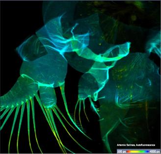
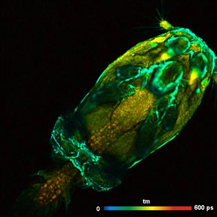
Artemia Salinas, Autofluorescence, DCS-120 Confocal Salmon
Louse, bh FLIM on Sutter MOM microscope
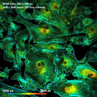
Bovine pulmonary artery cells, 560 nm, DCS-120
confocal Penicillium variabile, DCS-120 confocal
Bovine pulmonary artery cells, 480 nm, DCS-120
confocal Pig skin, stained with methylene blue, Zeiss LSM 880 NLO
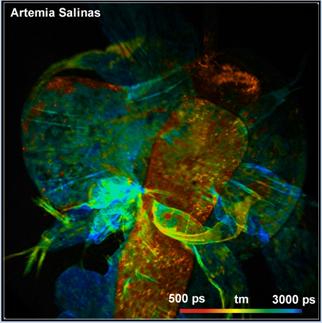
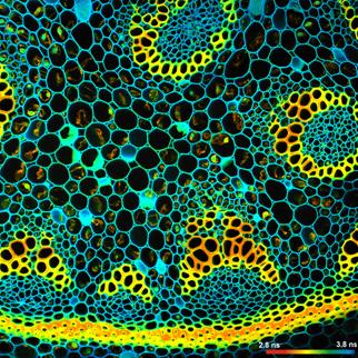
Artemia Salinas, Autofluorescence, DCS-120 MP
Convallaria sample, Zeiss LSM 780 NLO
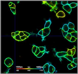
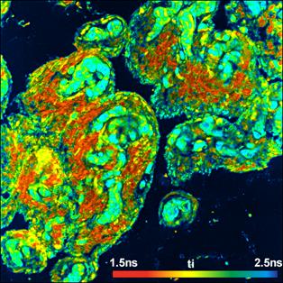
Membrane potential of HEK cells. Zeiss LSM 980 Pig
Skin, autofluorescence. Leica SP8 with HyD detectors
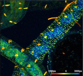
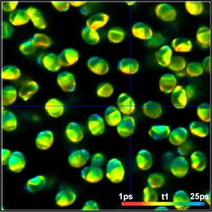
Enchytraeus
albidus, autofluorescence, 1 s aqusition time, Spores of paxillus
involutus. Ultra-fast decay.
DCS-120 with SPC-QC-104. Average
t1 is 12.5 ps. DCS-120 MP system.
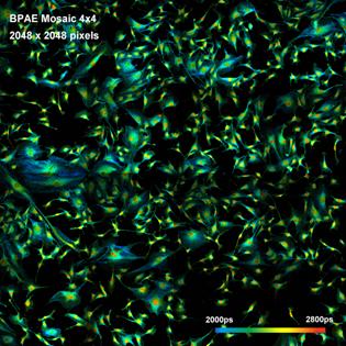
Mosaic FLIM image
of BPAE cell sample. DCS-120 MP FLIM Image recorded with DCS-120
MACRO system
1. W. Becker, Advanced time-correlated single-photon counting
techniques. Springer, Berlin, Heidelberg, New York, 2005
2. W. Becker, The bh TCSPC handbook, 9th edition. Becker & Hickl
GmbH (2019), available online on www.becker-hickl.com. Please contact bh for printed copies.
3. SPCImage NG data analysis software. In: W. Becker, The bh TCSPC
handbook, 9th edition. Becker & Hickl GmbH (2019)
4. W. Becker (ed.), Advanced time-correlated single photon counting
applications. Springer, Berlin, Heidelberg, New York (2015)
5. Becker & Hickl GmbH, DCS-120 Confocal and Multiphoton Scanning FLIM
Systems, user handbook 87th ed. (2019). Available on www.becker-hickl.com
6. Becker & Hickl GmbH, Modular FLIM systems for Zeiss
LSM 510 and LSM 710 family laser scanning microscopes. User handbook.
Available on www.becker-hickl.com
7. Becker & Hickl GmbH, FLIM systems from Zeiss LSM 980 Laser
scanning microscopes, addendum to modular FLIM systems for Zeiss LSM 510
and LSM 710 family laser scanning microscopes. Available on
www.becker-hickl.com
8. W. Becker, L. Braun, DCS-120 FLIM System Detects FMN in Live Cells.
Application note, available on www.becker-hickl.com
9. W. Becker, A. Bergmann, Precision fluorescence-lifetime Imaging of a
moving object. Application note, available on www.becker-hickl.com
10. W. Becker, A. Bergmann, M. Schubert, S. Smietana, Lifetime-intensity
mode delivers better FLIM images. Application note, available on
www.becker-hickl.com
11. Fast-Acquisition TCSPC FLIM: What are the Options? Application note,
available from www.becker-hickl.com
12. W. Becker, V. Shcheslavkiy, S. Frere, I. Slutsky, Spatially Resolved
Recording of Transient Fluorescence-Lifetime Effects by Line-Scanning TCSPC.
Microsc. Res. Techn. 77, 216-224 (2014)
13. R.M. Ballew, J.N. Demas, An error analysis of the rapid lifetime
determination method for the evaluation of single exponential decays, Anal.
Chem. 61, 30 (1989)
14. W. Becker, B. Su, K. Weisshart, O. Holub, FLIM and FCS Detection in
Laser-Scanning Microscopes: Increased Efficiency by GaAsP Hybrid Detectors.
Micr. Res. Tech. 74, 804-811 (2011)
15. Wolfgang Becker, Cornelia Junghans, Axel Bergmann, Two-photon FLIM
of mushroom spores reveals ultra-fast decay component. Application note,
available on www.becker-hickl.com.
16. Becker & Hickl GmbH, Ultra-fast HPM detectors improve NADH
FLIM. Application note, www.becker-hickl.com
17. Becker & Hickl GmbH, Two-Photon FLIM with a Femtosecond
Fibre Laser. Application note, www.becker-hickl.com
18. Becker Wolfgang, Suarez-Ibarrola Rodrigo, Miernik Arkadiusz, Braun
Lukas, Metabolic Imaging by Simultaneous FLIM of NAD(P)H and FAD. Current
Directions in Biomedical Engineering 5(1), 1-3 (2019)
19. H.C. Gerritsen, M.A.H. Asselbergs, A.V. Agronskaia, W.G.J.H.M. van
Sark, Fluorescence lifetime imaging in scanning microscopes: acquisition speed,
photon economy and lifetime resolution, J. Microsc. 206, 218‑224 (2002)
20. M. Köllner, J. Wolfrum, How many photons are necessary for
fluorescence-lifetime measurements?, Phys. Chem. Lett. 200, 199-204 (1992)
21. I. Isenberg, R.D. Dyson, The analysis of fluorescence decay by a
method of moments. Biophys. J. 9, 1337-1350 (1969)
Contact:
Wolfgang Becker
Becker & Hickl GmbH
Berlin, Germany
Email: becker@becker-hickl.com