Time-Tag Recording: A New Old Feature of the bh SPC Cards

‘Why don’t you implement time-tag recording in your TCSPC cards?’ This is one of the questions the bh user support is often asked. It is indeed hard to believe why we don’t: We cannot implement it because it is there - since 1996. The time-tag mode was first implemented in the SPC‑431 and -432 cards, one year later in the SPC‑630 cards. It is implemented in all currently available bh TCSPC modules, including the SPC‑134, SPC‑144, and SPC‑154 four-channel packages. Unfortunately, nobody talked about time-tagging in 1996, and so the mode was termed ‘FIFO Mode’.

Time-Tag Recording

Time-tag recording - or the ‘FIFO’ mode of the bh SPC cards - does not build up photon distributions but stores the full information about each individual photon. Each photon delivers three pieces of information: the time in the signal period, or ‘micro time, the number of the detector channel where the photon was detected, and the time from the start of the experiment, or ‘macro time’. These data are put into in a first-in-first-out (FIFO) buffer. During the measurement the FIFO is continuously read, and the photon data are stored in the main memory or on the hard disc of the computer [1]. The structure of a TCSPC device in the time-tag mode is shown in Fig. 1.

Fig. 1: Architecture of a bh TCSPC module in the FIFO mode

When a photon is detected, the ‘micro time’ in the signal period is measured by the time-measurement block. With the fast TAC/ADC principle used in the bh SPC modules the time is obtained with a channel resolution down to 820 femtoseconds. Simultaneously with the time measurement, the detector channel number for the current photon is written into the channel register. External events from the experiment, e.g. clock pulses from a scanner, may be read as well and put into the data stream. Moreover, each photon is tagged with the time from the start of the experiment. The macro time can be derived both from an internal clock oscillator and from a laser pulse sequence.

All the photon data - all in all four bytes per photon - are written into the FIFO buffer. The output of the FIFO is continuously read by the computer. The data can be processed online or offline, and decay functions, fluorescence correlation curves, photon counting histograms, MCS traces or BIFL data can be built up. Typical applications are described in [3, 5, 6, 7, 8].

The FIFO mode principle shown in Fig. 1 has similarity with the photon distribution modes of multi-dimensional TCSPC [1, 2]. In fact, the FIFO mode uses the same general building blocks within the TCSPC module. The channel register and the time measurement block are identical, the on-board memory is used as a FIFO buffer, and the sequencer block is used as a macro timer. In other words, all currently available bh TCSPC modules have both the photon distribution and the time-tag mode implemented, and the configuration is changed by a software command [2].

How to Use Time-Tag Recording

To use time-tag recording, open the ‘System parameters’, click into ‘Operation Mode’, and select the ‘FIFO’ mode as shown in Fig. 2, left.

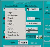
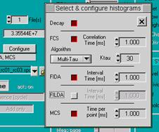
Fig. 2: Selection of the FIFO mode (left) and definition of the online-display (right)

With the FIFO mode selected you will obtain time-tag data but not necessarily see how the results build up during the measurement. To define online calculation and online display of the results, click into ‘Configure’. This opens the panel shown in Fig. 2, right. The available on-line functions are

-   Calculation of decay curves for the individual detectors

-   FCS by a multi-t algorithm or by a linear-t algorithm with subsequent binning. The maximum time up to which the correlation is calculated is defined by ‘Correlation Time’.

-   Calculation of photon counting histograms for the individual detectors (‘FIDA’). The sampling time interval is specified on the right.

-   Calculation of lifetime histograms (FILDA) for all detectors. The sampling time interval is specified on the right.

-   Intensity traces (MCS) for the individual detectors.

For all functions individual display windows are provided in the main panel, see Fig. 4.

For definition of correlation and cross correlation, configure the ‘Trace Parameters’ of the corresponding window to display the appropriate ‘Curves’ as shown in Fig. 3. ‘Curve’ defines the detectors FCS of which are to be calculated and displayed. ‘Cross-FCS Curve’ defines the detector number to correlate with. If ‘Curve’ and ‘Cross-FCS Curve’ are the same the autocorrelation is calculated. For different numbers the cross-correlation of the corresponding detectors is calculated. The configuration shown in Fig. 3 calculates the decay functions (histograms) of detector 1 and 2, the autocorrelation of  detector 1 and 2, and the cross-correlation of detector 1 and 2. In dual-module system you can also define cross-correlation betwenn detectors connected to different SPC modules.

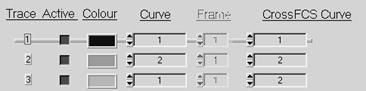
Fig. 3: Trace Parameters for the FCS display of FIFO mode

On-line calculation of correlation functions requires a considerable amount of computing power. This can slow down the display sequence below the specified ‘Display Time’ period. Moreover, the run-time calculations may dramatically reduce the readout rate from the SPC module. This is no problem for modules with large FIFO size and fast bus interface, such as the SPC-830 and SPC‑150 or ‑154. However, for the SPC-630 and the SPC-134 the on-line display can limit the count rates to 30 to 50 kHz. Therefore, do not calculate more fucntions than necessary, and make sure that the FIFO does not overflow when you use the on-line display. For the same reasons, the software is only able to calculate one correlation function per detector channel. If the Trace Parameters define several correlation functions for one channel, e.g. an autocorrelation and a cross-correlation with another channel, only the first correlation is calculated during the measurement. The other ones are calculated and displayed after the measurement is completed. Please see [2] for details.

Configuration of the SPCM Main panel

The main panel of the SPCM data acquisition software can be configured by the user. Two typical configurations for time-tag experiments are shown in Fig. 4.

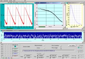
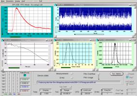
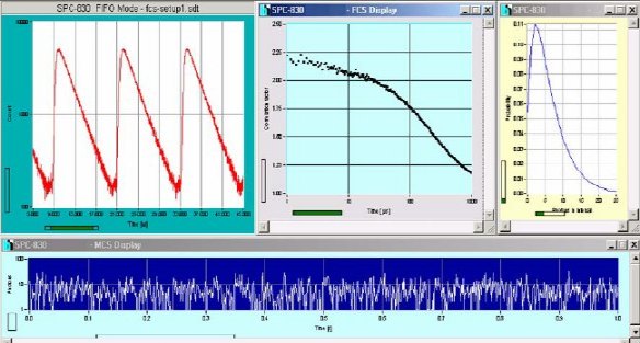
Fig. 4: Main panel of the SPCM software, examples of different configurations. The display windows show decay curves, FCS curves, photon counting histograms and intensity (MCS) traces.

Source of the Macro Time Clock

The bh SPC-830, SPC-130/134, SPC‑140/144 and SPC-150/154 provide an optional clock path from the SYNC input (normally the reference pulses from the laser) to the macro time clock. The SYNC clock avoids interference of the macro time clock period with the laser period. Moreover, it can be used to synchronise two SPC modules. Synchronised modules can be used to obtain FCS down to the SYNC period or, if the micro times are included, even down to the ps range [4]. The source of the macro time clock is selected via the ‘More Parameters’ button. Clicking on this button opens the panel shown in Fig. 5.

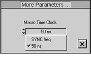
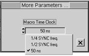
Fig. 5: Selection of the macro time clock source. Left: SPC‑830. Right: SPC‑130/134, ‑140/144 and ‑150/154

References

1.    W. Becker, Advanced time-correlated single-photon counting techniques. Springer, Berlin, Heidelberg, New York, 2005

2.    W. Becker, The bh TCSPC handbook. Becker & Hickl GmbH (2005), www.becker-hickl.com

3.    W. Becker, A. Bergmann, E. Haustein, Z. Petrasek, P. Schwille, C. Biskup, L. Kelbauskas, K. Benndorf, N. Klöcker, T. Anhut, I. Riemann, K. König, Fluorescence lifetime images and correlation spectra obtained by multi-dimensional TCSPC, Micr. Res. Tech. 69, 186-195 (2006)

4.    S. Felekyan, R. Kühnemuth, V. Kudryavtsev, C. Sandhagen, W. Becker, C.A.M. Seidel, Full correlation from picoseconds to seconds by time-resolved and time-correlated single photon detection, Rev. Sci. Instrum. 76, 083104 (2005)

5.    M. Prummer, C. Hübner, B. Sick, B. Hecht, A. Renn, U.P. Wild, Single-molecule identification by spectrally and time-resolved fluorescence detection, Anal. Chem. 72, 433-447 (2000)

6.    M. Prummer, B. Sick, A. Renn, U.P. Wild, Multiparameter microscopy and spectroscopy for single-molecule analysis, Anal. Chem. 76, 1633-1640 (2004)

7.    J. Schaffer, A. Volkmer, C. Eggeling, V. Subramaniam, G. Striker, C.A.M. Seidel, Identification of single molecules in aqueous solution by time-resolved fluorescence anisotropy, J. Phys. Chem. A 103, 331-336 (1999)

8.    F. Stefani, K. Vasilev, N. Bochio, F. Gaul, A. Pomozzi, M. Kreiter, Photonic mode density effects on single-molecule fluorescence blinking. New Journal of Physics 9 (2007)