The bh TCSPC Technique

Principles and Applications

Wolfgang Becker

Becker & Hickl GmbH, Berlin, Germany

Abstract: Starting from a discussion of the peculiarities of high-resolution low-level optical signal recording, this article describes the recording process of classic TCSPC and its extension, multi-dimensional TCSPC. It shows why TCSPC reaches a time resolution, sensitivity, and photon efficiency beyond the reach of any other optical signal recording technique. The article then passes to the general features of the bh TCSPC technique: Outstanding time resolution, outstanding timing stability, and a unsurpassed variety of multi-dimensional recording principles. These features are demonstrated on examples of high-resolution fluorescence decay recording, multi-detector operation and laser multiplexing, simultaneous fluorescence and phosphorescence recording, parameter-tag recording, FLIM, multi-wavelength FLIM, spatial and temporal mosaic FLIM, and simultaneous FLIM/PLIM.

Introduction

Time-correlated single photon counting (TCSPC) is an amazingly sensitive technique for recording low-level light signals with extremely high time resolution and extremely high precision. It is based on the detection of single photons, the measurement of the times of the photons after the reference (usually excitation) pulses, and the construction of the waveform of the optical signal from the photon times [12, 44].

TCSPC has been derived from the delayed coincidence method for the measurement of excited nuclear state lifetimes [29]. The technique has been used since the 60s of the last century. For many years TCSPC was used primarily to record fluorescence decay curves of organic dyes in solution [31, 39, 40, 50, 53]. Due to the low intensity and low repetition rate of the light sources and the limited speed of the electronics of the 70s and 80s the acquisition times were extremely long. More important, classic TCSPC was intrinsically one-dimensional, i.e. limited solely to the recording of the waveform of the light signal.

Light sources ceased to be a limitation when the first mode-locked Argon lasers and synchronously pumped dye lasers were introduced. For the recording electronics, the situation changed with the introduction of the SPC-300 modules of Becker & Hickl in 1993. Due to a new Time-to-Amplitude and Analog-to-Digital Conversion (TAC/ADC) principle these modules worked at photon count rates almost 100 times higher than previous TCSPC devices. Time resolution (or IRF width) improved from about 50 ps for classic devices to 15 ps for the SPC-300. Currently, the fastest bh TCSPC modules reach <3 ps (FWHM) internal IRF width, and a time-channel width down to 203 femtoseconds.

Another novelty introduced by bh was the extension of the classic TCSPC process to multi-dimensional recording. Already the SPC-300 and SPC-330 modules recorded photon distributions not only over the time in a fluorescence decay but simultaneously over the wavelength of the photons or over a spatial coordinate. Within a few years, bh added more and more dimensions to multidimensional TCSPC. Fast sequential recording was introduced with the SPC-430 in 1995, fast scanning with the SPC-535 in 1996. Time-tag recording was introduced with the SPC-431 in 1996. FLIM for laser scanning microscopy was introduced in 1999. Since then, the bh TCSPC systems became bigger, faster and more complex. Recent TCSPC modules can be configured for sequential recording, imaging, or time-tag recording by a simple software command. They can run classic TCSPC experiments, FLIM, multi-wavelength FLIM, spatial and temporal mosaic FLIM, FLITS, and simultaneous FLIM/PLIM. Multi-module systems, like the bh SPC‑154, the bh Max‑Tau 12‑channel system, or the bh FASTAC FLIM system, can be used for recording at unprecedented count rates and acquisition speeds without compromise in time resolution.

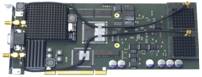
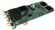
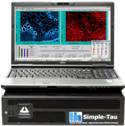
Fig. 1: SPC-150NX TCSPC/FLIM module, SPC-180 TCSPC/FLIM Module, Simple-Tau 152 dual-channel TCSPC/FLIM system

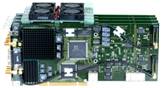
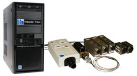
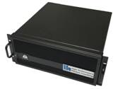
Fig. 2: SPC-154 four-channel TCSPC/FLIM module, Power-Tau 4-channel TCSPC system, MAX-Tau 12 Channel TCSPC system

The TCSPC Recording Process

Detection of Low-Level Light Signals

Time-correlated single photon counting, or TCSPC, is based on the detection of single photons of a periodic light signal, the measurement of the detection times of the photons, and the reconstruction of the waveform from the individual time measurements [12, 44]. TCSPC makes use of the fact that for low-level, high-repetition rate signals the light intensity is low enough that the probability to detect more than one photon in one excitation pulse period is negligible. The situation is illustrated in Fig. 3.

Fig. 3: Detector signal for fluorescence detection at a pulse repetition rate of 80 MHz

Fluorescence of a sample is excited by a laser of 80 MHz pulse repetition rate (a). The expected fluorescence waveform is (b). However, the detector signal, (as measured by an oscilloscope) has no similarity with the expected fluorescence waveform. Instead, it is a sequence of extremely narrow pulses randomly spread over the time axis (c). A signal like this often looks confusing to users not familiar with photon counting. However, there is a simple explanation: The pulses represent single photons of the light signal arriving at the detector. The shape of the pulses has nothing to do with the waveform of the light signal. It is the response of the detector to the detection of a single photon.

The Classic TCSPC Process

There are two conclusions from the signal shape in Fig. 3 (c). First, the waveform of the optical signal is not the detector signal. Instead, it is the distribution of the detector pulses over the time in the excitation pulse periods. Second, the detection of a photon within a particular excitation pulse period is a relatively unlikely event. The photon detection rate of (c) was about 10⁷ s^-1. This is close to the maximum permissible count rate of most single-photon detectors. A detection rate of 10⁷ s^-1 means that the probability to detect a photon in one 80 MHz period is 0.125. The probability to detect two photons is 0.0156, the detection of more photons is even less likely. Therefore, only the first photon within a particular pulse period has to be considered. The build-up of the photon distribution over the pulse period then becomes a relatively straightforward process.

The principle is illustrated in Fig. 4, left. When a photon is detected, the arrival time of the corresponding detector pulse in the signal period is measured. The detection events are collected in a memory by adding a 1 at an address proportional to the detection time. After many signal periods a large number of photons has been detected, and the distribution of the photons over the time in the signal period has been built up. The result represents the waveform of the optical pulse.

Multi-Dimensional TCSPC

All bh TCSPC modules are able to work by the classic TCSPC process. However, the bh TCSPC devices are able to do much more than that. Unlike classic TCSPC devices, they can record photon distributions not only over the time in the excitation pulse period, but also over additional parameters that are associated to the individual photons. This can be the wavelength of a photon, the spatial location where it came from, the time from the start of an experiment, the time within the period of a stimulation of the sample, the time within the period of a modulation of the excitation laser, or any other parameters that are determined or actively controlled during the recording process [12, 16, 17]. The multi-dimensional TCSPC process is illustrated in Fig. 4, right.

Fig. 4: Left: Classic TCSPC records a distribution over the times of the photons after the excitation pulses. Right: Multi-dimensional TCSPC records a photon distribution over the photon times and one or several other parameters, here the wavelength of the photons.

By having both classic and multi-dimensional TCSPC implemented, the bh SPC devices work for the classic fluorescence decay applications as well as for anti-bunching experiments, simultaneous fluorescence and phosphorescence decay measurement, multi-wavelength fluorescence decay measurement, fluorescence lifetime imaging (FLIM), multi-wavelength FLIM, simultaneous FLIM and PLIM, ultra-fast time-series fluorescence decay recording, fast time-series FLIM, fluorescence correlation (FCS), single-molecules experiments, and other multi-dimensional photon recording tasks. Please see [16] for examples and applications.

Key Parameters of a TCSPC System

High Photon Efficiency - High Lifetime Accuracy

In a TCSPC device operated at reasonable count rate all detected photons contribute to the result. There is no suppression of photons due to gating as in Boxcar devices or gated image intensifiers, and no variable weight as in sine-wave modulation techniques. TCSPC therefore reaches a near-ideal photon efficiency.

The high photon efficiency of TCSPC translates directly into the accuracy for fluorescence lifetime recording. Under ideal conditions a single-exponential fluorescence lifetime can be determined at a signal-to-noise ratio, SNR, of

from a number of detected photons, N. TCSPC comes very close to the theoretical SNR [1, 37]. In combination with the fact that TCSPC delivers the shortest possible IRF for a given detector (see below) it yields the best possible lifetime accuracy (or Photon Efficiency) for a given number of detected photons [1, 37 Ballew, Köllner].

Time Resolution

Different than for an analog-recording technique, the time resolution of TCSPC (both classic and multi-dimensional) is not limited by the single-photon response of the detector. Instead, it is given by the transit time jitter, or transit-time spread, of the detector-TCSPC combination, see Fig. 5. The transit time spread is much shorter than the width of the single-photon response. The difference can be enormous, as shown in Fig. 6 for a fast hybrid detector. The single-photon response of the detector is about 1 ns wide (Fig. 6, left). However, the transit time jitter is less than 20 ps, resulting in a correspondingly short TCSPC response (Fig. 6, right, note different time scale).

Fig. 5: Single-photon response of detector and instrument response function (IRF) of a TCSPC system. The IRF width is given by the transit-time spread, not by the width of the single-photon response of the detector.

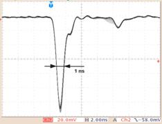
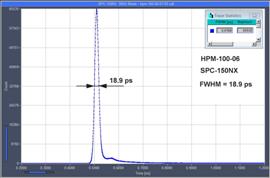
Fig. 6: Single electron response (SER, left) and TCSPC Instrument response function (IRF, right) for a bh HPM-100‑06 hybrid detector. The TCSPC IRF is more than 50 times faster than the SER. Note the different time scale.

The distribution of the recording events over the time after a reference pulse for an infinitely short light pulse is called the Instrument Response Function, or IRF. Please note that there are different parameters to describe the time resolution of a TCSPC system: The FWHM (Full Width at Half Maximum) describes the width of the IRF, the RMS (Root Mean Square) describes the average timing jitter, or the standard deviation of the photon times. For near-Gaussian IRF shapes the RMS jitter value is 2.5 to 3 times smaller than the FWHM of the IRF.

Time-Channel Width

Signal theory demands the IRF to be sampled with a density of data points that yields at least 10 data points on the IRF. Only then the full information can be extracted from the recorded signals. Small time-channel widths (or high effective sampling rates) can easily be obtained by TCSPC, but not by analog-recording techniques. Please note that the time-channel width is sometimes specified as time resolution. This is wrong - the true time resolution is given by the FWHM of the IRF or the RMS timing jitter. Oversampling a broad IRF with a large number time channels does not result in real time resolution.

Timing Stability

In many instances, timing stability (including low-frequency timing wobble) is even more important than time resolution. Examples are distance measurements and diffuse-optical imaging applications, where changes in the mean time-of-flight of the photons on the order of a few ps are recorded over tens of minutes. Even in standard fluorescence-decay measurements timing drift matters: Timing shift between the fluorescence recording and a related IRF recording transfers directly into the measured fluorescence lifetime. Moreover, there are setups where an exact IRF is difficult to record. Typical examples are confocal microscopes where dichroic mirrors and filters block the detection path for the excitation wavelength. In these cases, it is important that a stable IRF is maintained over a long period of time. The bh TCSPC technique addresses these issues by extraordinarily low timing drift and timing wobble, please see section below.

Maximum Count Rate

Both the classic and the multidimensional TCSPC process require that the photon rate is lower than the excitation pulse rate. This requirement and possible Pile-Up errors induced by high detection rate are constant subject of controversy. We have, however, shown that detection rates of up to 10% of the excitation pulse rate can be used without inducing noticeable errors. In practice, the count rate is rather limited by the photostability of the sample than by the pile-up limit of the TCSPC technique.

Another controversial parameter is the Dead Time of a TCSPC device. Dead time is the time the device needs to process a single photon. If a new photon is detected within this time it is not recorded. Consequently, there is a Counting Loss which increases with the detector count rate. However, dead time (within reasonable limits) has also positive effects. It helps suppress afterpulses of the detectors, and it avoids an influence of the recording of a photon on the timing of the next one. The dead time prevents the recording of photons that are too close to each other and thus helps maintain a high time resolution and a high IRF stability over a wide range of count rates. Please see [12] and [16] for details.

Reversed Start-Stop

TCSPC techniques of the 1960s and 1970s determined the photon times from the excitation pulse to the photon. With the introduction of excitation sources with pulse periods of 8 to 12 ns the timing was reversed [36]. The reason is that it is technically difficult, if not impossible, to start a time-measurement cycle every 8 ns, reset the circuitry if no photon was detected, and start it again. Recent TCSPC devices therefore start the time measurement with the photon, and measure the time to the next excitation pulse or to the delayed excitation pulse [12, 16].

General Features of the bh TCSPC Devices

Electrical IRF

The bh SPC-150N, SPC-160N, and SPC-180N series devices use a patented high-speed high-resolution TAC/ADC principle [12, 16]. The internal timing jitter is on the order of 2 to 3 ps (rms) for the standard modules, 1.6 ps for the SPC-150NX modules, and 1.1 ps (rms) for the SPC-150NXX boards, see Fig. 7. The FWHM IRF widths are 6.8 ps, 3.5 ps, and <3 ps, respectively. This is much better than for any TCSPC device based on direct time-to-digital conversion (TDC) [4], and significantly smaller than the timing jitter of the commonly used detectors. Moreover, the signals are sampled with a sufficient number of sufficiently small time channels: The minimum time-channel width for the standard SPC-N boards is 810 fs, 405 fs for the SPC-NX board, and 202 fs for the SPC-NXXs board. It is thus possible to resolve extrely fast decay processes [26]. Please note that a 202-fs time-channel width is equivalent to a sampling rate of 5 THz!

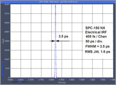
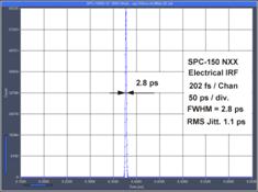
Fig. 7: Electrical IRF of an SPC-150NX (left) and SPC-150NXX (right)

IRF with Fast Detectors

Due to their short electrical IRF and small time-channel width the bh TCSPC modules deliver unprecedented system IRF widths with fast photon detectors. The FWHM instrument response width for fast hybrid detectors, MCP PMTs and superconducting NbN detectors is in the sub-20 ps range [2, 3]. With single-nanowire NbN detectors less than 5 ps IRF width have been achieved [21]. Examples are shown in Fig. 8.

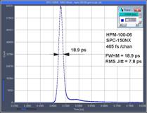
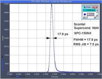
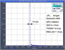
Fig. 8: Instrument response functions for a fast hybrid detector, a superconducting NbN detector, and a superconducting single-nanowire detector.

Timing Stability

Different than TCSPC devices based on TDCs, the bh devices are virtually free of IRF drift or low-frequency timing wobble. IRF drift, if perceptible at all, remains below the electrical IRF width over minutes or even hours. That indirectly means that the IRF neither broadens in an experiment of long acquisition time nor shifts over a longer series of recordings. Fig. 9, left and right, shows a series of 100 IRF recordings over 100 seconds. The horizontal axis is the TCSPC time axis, the vertical axis is the time into the series. The variance in the time of the IRF centroid is less than 0.4 ps. Overall timing drift of a real measurement system is shown in Fig. 10. It shows two IRFs of an SPC-150NX system with a superconducting NbN detector, recorded 5 minutes apart. The timing drift is less than the time-channel width (405 fs for this measurement).

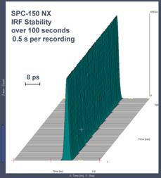
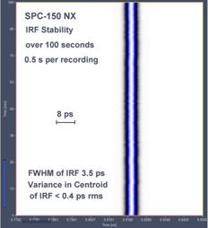
Fig. 9: Series of 100 (electrical) IRF recordings over 100 seconds. Left: Result displayed as series of curves. Right: Colour-Intensity display. The horizontal axis is the TCSPC time axis (bar indicates 8 ps), the vertical axis is the time into the recording sequence. The variance in the centroid of the IRF is less than 0.4 ps rms.

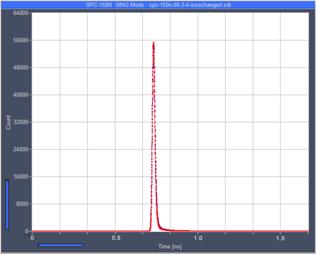
Fig. 10: Two IRFs of a TCSPC system with a superconducting NbN detector, recorded 5 minutes apart (black and red dots). The drift is less than one time-channel (405 fs).

Application: High-Resolution Fluorescence-Decay Recording

The most frequent application of classic TCSPC is fluorescence-decay recording. A sample is excited with a high-frequency pulsed laser, and the fluorescence decay functions are recorded by TCSPC.

With their short IRF functions and high timing stability, bh TCSPC devices record high-quality decay curves at extremely high time resolution [16]. Fig. 11 shows the fluorescence decay of a rhodamine dye. The fluorescence was excited by a bh BDS-405 picosecond diode laser, the photons were detected by a HPM-100-06 ultra-fast hybrid detector. When the fluorescence decay is recorded over an interval of 0 to 50 ns (Fig. 11, left) the IRF width is almost invisible. A recording at a faster time scale (Fig. 11, right, 0 to 5 ns) shows that the IRF is about 40 ps wide. It is essentially determined by the laser pulse width, which was approximately 35 ps. In the 0 to 5 ns interval, the fluorescence almost looks like phosphorescence.

The fluorescence decay of an infrared dye recorded with a superconducting single-nanowire detector [21] is shown in Fig. 12. At first glance, the curve may look like a decay curve of fluorescein recorded in a standard lifetime spectrometer. In fact, the IRF width is 5 ps FWHM, and the decay time is 43.7 ps, i.e. almost 100 times shorter than that of fluorescein.

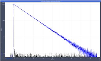
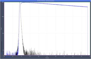
Fig. 11: Left: Fluorescence decay of a rhodamine dye recorded with a bh ps diode laser, a fast hybrid detector, and a bh SPC-150N TCSPC module. Logarithmic scale, time axis 0 to 50 ns. Right: Same signal recorded in a time range of 0 to 5ns.

Fig. 12: Fluorescence decay of an infrared dye, recorded with a femtosecond laser, a single-nanowire superconducting NbN detector, and an SPC-150NXX TCSPC module. The IRF width is 5 ps, a fit of the data with a single-exponential model function delivers a fluorescence decay time 43.7 ps.

Routing

The term Routing refers to the ability of the TCSPC device to route photons into different measurement data blocks depending on an external control signal. The routing function can be used to record signals from several detectors by a single TCSPC device, to separate photons excited by several multiplexed lasers, or to record photons from spatially different positions of an object by fast optical switches [16]. Routing has already been introduced in the classic-TCSPC era. It is, however, an important element of multi-dimensional TCSPC: The photons are assigned one or more additional parameters (detection channel, excitation wavelength, spatial position), and the result is a photon distribution over the time in the optical waveform and these parameters.

Application: Dual-excitation and dual-emission wavelength recording of decay curves

An example of dual-detector and dual-laser operation is shown in Fig. 13. Two lasers were multiplexed at a rate of 20 Hz, and the photons detected by two detectors through different filters. The result contains three decay curves for different excitation/detection wavelength combinations. The fourth combination does not deliver data because the detection wavelength is shorter than the excitation wavelength. Please see [16] for further details.

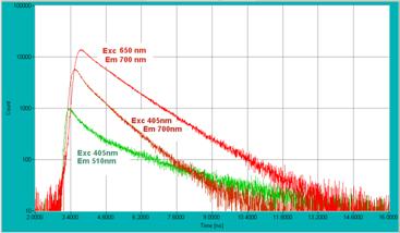
Fig. 13: Multiplexed measurement of the fluorescence of a leaf. Multiplexed excitation at 405 nm and 650 nm, simultaneous detection at 510 nm and 700 nm. Multiplexing rate 20 Hz.

Dual Time-Base Recording

The bh TCSPC modules can associate two times to every individual photon. The first one, the micro time is the time in the excitation pulse period. This is the usual TCSPC time, and it is available at an accuracy in the ps range. The second time, the macro time, is a time from the start of the experiment or from an external event. The capability to associate two times to the photons results in recording principles which are beyond the reach of classic TCSPC. Two examples are described below, for details and more applications please see [16].

Application: Simultaneous Fluorescence and Phosphorescence Decay Recording

The technique is based on on-off modulating a high-frequency pulsed laser and recording the fluorescence and phosphorescence signals by dual time-base TCSPC. The fluorescence decay is obtained by building up a photon distribution over the times of the photons in the laser pulse period (the micro times), PLIM by building up the distribution over the times of the photons in the laser modulation period (the macro times) [16]. The modulation and photon timing principle is illustrated in Fig. 14. An example is shown in Fig. 15. Please see also Simultaneous FLIM / PLIM, page 24.

Fig. 14: Modulation and photon timing for simultaneous fluorescence and phosphorescence decay recording

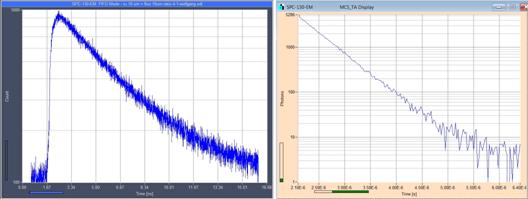
Fig. 15: Simultaneous recording of fluorescence (left) and phosphorescence decay (right). Mixture of fluorescein and a ruthenium dye.

Application: FCS

Fluorescence Correlation Spectroscopy (FCS) is based on the recording of fluorescence from a limited number of fluorescing molecules in a small sample volume, and correlating intensity fluctuations caused by the motion of the molecules [13, 45]. The correlation curves are calculated by

where G(t) is the autocorrelation function of a single signal, I(t), and G₁₂(t) the cross-correlation function of two signals, I₁(t) and I₂(t). N(t) is the photon number in a given macro-time interval. A correlation curve of a fluorescein solution is shown in Fig. 16.

FCS can be combined with fluorescence decay recording. The decay curves are obtained by building up the photon distribution over the micro times of the photons. Please see [16] for more information.

LvG

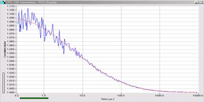
Fig. 16: FCS curve recorded with bh SPC-150 module and HPM‑100-40 hybrid detector. FCS curve calculated online by SPCM software. The red curve is a fit with a two-component diffusion model.

Recording of Parameter-Tagged Photons

The TCSPC processes described above build up photon distributions in the memory of the TCSPC device or transfer the single-photon data into the system computer which immediately builds up the photon distributions. Once a photon has been put in the photon distribution the information associated to it is no longer needed and, normally, discarded.

Parameter-tagged photon data may, however, be used to build up other results than multi-dimensional photon distributions. At the time of the experiment it may even not be clear how exactly the photon data are to be processed. User-interaction during the data processing may be required, or the processing may require so much computation power that it cannot be performed online. In these cases the single-photon data (micro time, macro time, routing information, markers for external events) can be saved for later off-line processing [12, 16, 17]. Most of the applications of parameter-tag recording are in the field of single-molecule spectroscopy. An example is described below.

Application: Single-Molecule Burst Analysis

Consider a solution of fluorescent molecules, excited by a focused laser beam through a microscope lens, with the emitted photons being detected through a confocal pinhole that transmits light only from a volume of diffraction limited size. When the concentration of fluorescent molecules is low enough only one molecule will be in the detection volume at a time. As the molecule diffuses through the excitation/detection volume it emits photons. Thus, the detection signal consist of bursts of photons caused by individual molecules, see Fig. 17.

Fig. 17: Photon bursts from single molecules travelling through a femtoliter-size detection volume

For single-molecule analysis, the single-photon data stream from the TCSPC module is stored, the bursts from the individual molecules are identified in the data, and multi-dimensional histograms of the fluorescence parameter values are built up. It is even possible to record changes in the fluorescence parameters within the individual bursts, derive FRET efficiencies, and conclude on conformational changes of the molecules [42, 52]. Please see [16], chapter Multi-Parameter Single-Molecule Burst Analysis.

Multi-Dimensional TCSPC Techniques

Multi-Wavelength Recording

Multi-wavelength TCSPC is based on splitting the light spectrally into a number of detector channels (or channels of a multi-anode PMT), and using the number of the channel the photon arrived at as a second coordinate of the photon distribution [7, 14]. The principle is shown in Fig. 18. For each photon, the detector delivers a single-photon pulse which indicates the detection time, and a Channel signal which indicates in which channel of the multi-anode PMT the photon arrived. The TCSPC module builds up a photon distribution over the photon time and the channel number. The result is identical with a set of decay curves (in this case 16) for different wavelengths.

Fig. 18: Principle of multi-wavelength TCSPC

Application: Multi-Wavelength Fluorescence Decay Recording

Please note that multi-wavelength TCSPC does not use any wavelength scanning, detector switching, or multiplexing. Every photon is put into a place in the photon distribution according to its detection time and wavelength. Compared to scanning the spectrum with a monochromator and recording individual decay curves, the efficiency is much higher. Multi-detector TCSPC, especially multi-wavelength detection, has therefore become a commonly used technique of autofluorescence lifetime imaging of biological samples [30, 41, 46]. An example is shown in Fig. 19.

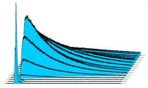
Fig. 19: Multi-wavelength fluorescence-decay recording. PML-16 GaAsP multi-wavelength detector with SPC‑150 TCSPC module. The peak on the lower left is the excitation light.

Ultra-Fast Time Series Recording

Multi-dimensional TCSPC is able to record ultra-fast time series of fluorescence decay curves. The process is based on a periodic induction of a dynamic effect in the sample and recording a two-dimensional photon distribution over the times of the photon after the excitation pulses and after the stimulation of the sample [16].

Application: Recording of Chlorophyll Transients

As an example, Fig. 29 shows the photochemical transient of chlorophyll in a plant. Stimulation was performed by periodically switching on and off the excitation laser. Time per curve is 100 microseconds - a speed impossibly to be obtained by classic TCSPC.

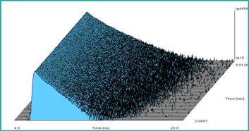
Fig. 20: Ultra-high speed time-series recording. Photochemical chlorophyll transient in a leaf, sequence of 128 decay curves, 100 µs per curve.

Fluorescence Lifetime Imaging (FLIM)

FLIM by multi-dimensional TCSPC is based on scanning a sample by the focused beam of a high-repetition rate laser and detecting single photons of the fluorescence signal. Each photon is characterised by its time in the laser period and the x-y position of the laser spot in the moment of the photon detection. The recording process builds up a photon distribution over these parameters [12, 15, 16, 17]. The principle is illustrated in Fig. 21. The result is an array of pixels, each containing a full fluorescence decay curve with a (typically large) number of time channels. The process works at any scan rate, and delivers near-ideal photon efficiency and extremely high time resolution.

Fig. 21: Fluorescence lifetime imaging

An example of a FLIM image is shown in Fig. 22. A convallaria sample was scanned with a bh DCS-120 confocal scanner [5]. The excitation source was a BDL-SMN 473-nm ps diode laser, the photons were detected by a bh HPM-100-40 hybrid detector and processed by an SPC-150 TCSPC/FLIM module. The data were recorded into 2048 x 2048 pixels and 256 time channels per pixel. The brightness of the image represents the photon number, the colour the fluorescence decay time. Decay curves for selected pixels shown on the right.

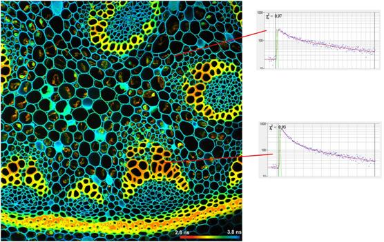
Fig. 22: FLIM image of a Convallaria Sample, 2048x2048 pixels, 256 time-channels per pixel. Decay curves for selected pixels shown on the right.

The bh devices record FLIM images with different scanning techniques and optical systems, and with image scales from nanometers (STED [8]), micrometers (confocal and multiphoton microscopy [11]) or millimeters and centimetres (bh macro scanner [47], clinical systems [51]). For more examples and references please see [5, 6, 16] and [18].

Application: FLIM-FRET

FRET, or Foerster Resonance Energy Transfer, is used in cell biology to study the interactions between proteins [43]. The proteins are labelled with a donor and an acceptor. When the donor is excited, the energy can be emitted via fluorescence or transferred to the acceptor. The energy transfer rate sensitively depends on the distance to the acceptor. In practice, FRET occurs only when the donor-labelled protein is chemically linked to the acceptor-labelled one. The energy transfer rate is a measure of the distance. Compared to intensity-based FRET techniques FLIM-FRET is much more reliable. All that is needed is a lifetime image at the donor emission wavelength. The decrease in the donor fluorescence lifetime then indicates the rate of the energy transfer. Another advantage is that interacting and non-interacting donor (or interacting and non-interacting proteins) can be separated by double-exponential decay analysis. It is thus possible to measure the fraction of interacting proteins. This is biological information not accessible by intensity-based FRET techniques. Please note that double-exponential analysis of FRET decays requires high time resolution. Therefore, the technique benefits considerable from the high time resolution of the bh TCSPC / FLIM devices. Please see FRET chapter in The bh TCSPC Handbook [16]. An example of double-exponential FLIM-FRET is shown in Fig. 23.

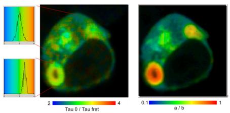
Fig. 23: FRET result obtained by double exponential lifetime analysis. Left: t₀/t_fret, indicating distance variation, Right: N_fret/N₀_, indicating variation in amount of interacting proteins.

Application: Metabolic Imaging

The composition of the decay curves of NADH (nicotimamide adanine (pyridine) dicucleotide) is an indicator of the metabolic state of cells and tissues. A high amplitude of the fast component (from free NADH) indicates the cells are running glycolysis, a low amplitude indicates that oxidative phosphorylation dominates [16]. It turns out that the amplitude of the fast component (or the amplitude ration of the fast and slow component) is a much better indicator of the metabolic state than the fluorescence lifetime itself [22]. However, the determination of the amplitudes requires double-exponential decay analysis, and, consequently, high resolution of the decay data. Metabolic FLIM therefore benefits from the high time resolution of the bh FLIM devices. An example is shown in Fig. 24 and Fig. 25. The sample was excited by two-photon excitation with a femtosecond Ti:Sa laser, the photons were detected by a HPM-100-06 ultra-fast hybrid detector. The result shows the best separation of the NADH decay components ever obtained. The data not only yield an excellent image of the amplitude-weighted mean lifetime, but also high-quality images of the amplitude ratio and the component lifetimes [10]. For clinical application please see [22, 23, 49].

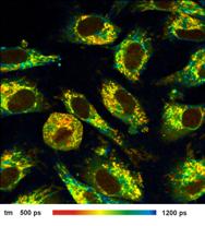
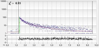
Fig. 24: Left: NADH Lifetime image, amplitude-weighted lifetime of double-exponential fit. Right: Decay curve in selected spot, 9x9 pixel area. FLIM data format 512x512 pixels, 1024 time channels. Time-channel width 10ps.

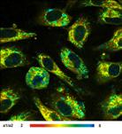
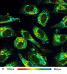
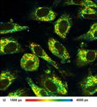
Fig. 25: Left to right: Images of the amplitude ratio, a1/a2 (unbound/bound ratio), and of the fast (t1, unbound NADH) and the slow decay component (t2, bound NADH). FLIM data format 512x512 pixels, 1024 time channels. Time-channel width 10ps.

Application: Ultra-Fast Fluorescence Decay in Biological Systems

With their short IRF bh FLIM systems are able to detect ultra-fast decay components which have never been seen before [24, 25, 26, 27]. An example is shown in Fig. 26.

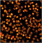
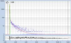
Fig. 26: Ultra-fast decay in mushroom spores, t₁ image and decay curve. The lifetime of the fast decay component is 12 ps.

Application: FLIM in Ophthalmology

TCSPC FLIM is so sensitive that it can be used to record fluorescence-lifetime images of the human retina. Examples are shown in Fig. 27. The images were recorded with the Heidelberg-Engineering FLIO system, containing bh TCSPC FLIM modules, bh ps diode lasers, and bh HPM hybrid detectors. Also here, time resolution and timing stability are extremely important: Fluorescence decay times range from 200 to 600 ps, with component lifetimes down to less than 80 ps. The problem is not only that the lifetimes are very short but also that the optical path length is not constant and that the retina signal is contaminated by fluorescence from the front part of the eye [28]. Technical details are described in [16] and [51]. Ophthalmic FLIM is currently under clinical trial. The results show that FLIM is able to detect early changes in the metabolism of the retina before these have caused irreversible damage. Please see [16], [28] and [32] for references.

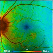
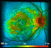
Fig. 27: Lifetime images of the human retina. Left: Healthy eye. Right: Eye of an AMD (age-related macula degeneration) patient.

Multi-Dimensional FLIM Techniques

The photon distribution of TCSPC FLIM can be extended by additional parameters. These can be the wavelength of the photons, the time from the start of the experiment or from a stimulation of the sample, the excitation wavelength, or the time in the period of an additional modulation of the excitation laser. The resulting photon distributions are four- or five-dimensional, the data representing multi-spectral FLIM, ultra-fast time-series FLIM, multi-excitation-wavelength FLIM, and simultaneous FLIM/PLIM. A few examples are shown in the sections below. Please see [16, 17, 18, 48] for more information.

Multi-Wavelength FLIM

Multi-wavelength (or multi-spectral) FLIM uses a combination of the FLIM architecture shown in Fig. 21 with multi-wavelength detection principle described in Fig. 18. In addition to the times of the photons and the positions, x, and y, of the scanner, the TCSPC module determines the detector channel that detected the photon. These pieces of information are used to build up a photon distribution over the time of the photons in the fluorescence decay, the wavelength, and the coordinates of the image [7, 14, 16, 17]. The result is an image that contains several decay curves for different wavelength in each pixel. An example of a multi-wavelength FLIM image is shown in Fig. 29.

Fig. 28: Multi-wavelength FLIM. The recording process builds up a photon distribution over x,y,t, and λ.

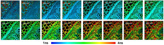
Fig. 29: Multi-wavelength FLIM of a convallaria sample

FLIM with Excitation-Wavelength Multiplexing

The routing function of the bh TCSPC modules can be used to record FLIM quasi-simultaneously at several excitation wavelengths. Several lasers are multiplexed synchronously with either the pixels, the lines, or the frames of the scan, and the photons excited by different lasers are routed into different FLIM data blocks. The result represents separate lifetime images for the individual laser wavelengths [16]. The principle is shown for two lasers in Fig. 30.

Fig. 30: Principle of TCSPC FLIM with laser wavelength multiplexing

Excitation-wavelength multiplexing is often combined with detection in several emission wavelength intervals via several parallel TCSPC modules or a router. The result is then a data set which contains FLIM images for all combinations of excitation and detection wavelengths [22].

Application: Metabolic FLIM with NADH and FAD

Although the fluorescence of NADH is the best metabolic indicator also FAD (flavin adenine dinucleotide) exhibits changes in its decay behaviour with the metabolic state of a cell. Lifetime images of FAD are therefore often used to support the metabolic information obtained from NADH. The problem of this approach is that NADH and FAD data are desirably to be recorded simultaneously. Unfortunately, NADH and FAD signals can only be separated if both different excitation and detection wavelengths are used. The task can be solved by the excitation multiplexing principles shown above. A result is shown in Fig. 31. The data were recorded by a bh DCS-120 system with two lasers, 375 nm and 410 nm, and two TCSPC / FLIM channels, detecting from 420 nm to 470 nm and 490 nm to 600 nm, respectively [5]. Technical details and the discrimination of healthy cells and tumor cells are described in [22, 23, 49].

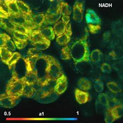
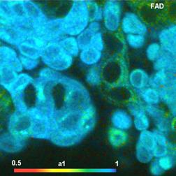
Fig. 31: a₁ Images of human bladder cells, recorded with two multiplexed lasers and two TCSPC channels.

Mosaic FLIM

Originally, bh introduced Mosaic FLIM to record large images with the Tile Imaging function of laser scanning microscopes [6, 16]. The microscope scans the sample, and performs a raster stepping (Tile stepping) of the sample. For every step the sample is scanned for a defined number of frames. The TCSPC device records the data by its normal FLIM procedure. However, the memory is configured to provide space not only for a single image of the defined frame format but for the entire mosaic of images of the tile stepping. The TCSPC FLIM process starts in the first mosaic element. After a defined number of frames the recording proceeds to the next mosaic element. Provided the number of frames per tile of the microscope stepping and the number of frames per mosaic elements are the same the TCSPC module records the entire tile array into a single photon distribution. The recorded photon distribution represents a FLIM image of the entire array. The TCSPC FLIM process of Mosaic FLIM is illustrated in Fig. 32. An example is shown in Fig. 33.

Fig. 32: Mosaic FLIM, recording of a X-Y mosaic

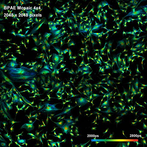
Fig. 33: Mosaic FLIM of a BPAE cell sample

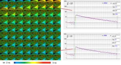
Temporal Mosaic FLIM

The idea that Mosaic FLIM records several images into one photon distribution leads to a more general concept of Mosaic FLIM: The transition from one mosaic element in the FLIM data to the next can be associated also to a change in another parameter of the experiment. An example is temporal mosaic FLIM. The sample is repeatedly scanned around the same spatial position, but subsequent images are recorded in consecutive elements of the FLIM mosaic. The result is a time series, the time step of which is a multiple of the frame time [16].

Compared to conventional time-laps recording the temporal mosaic FLIM has several advantages: No time has to be reserved for the save operations, and the data can be better analysed with global-parameter fitting. The biggest advantage is, however, that mosaic time series data can be accumulated: A sample would be stimulated repeatedly by an external event, and the start of the mosaic recording be triggered with the stimulation. With every new stimulation the recording procedure runs through all elements of the mosaic, and accumulates the photons. Accumulation allows data to be recorded without the need of trading photon number and lifetime accuracy against the speed of the time series. Consequently, the time per step (or mosaic element) is only limited by the minimum frame time of the scanner.

Application: Recording of Calcium Transients in Neurons

Temporal Mosaic FLIM is thus an excellent way to investigate fast physiological processes in live systems [20, 33]. An example for recording Ca²⁺ transients in live neurons is shown in Fig. 34. Please see [16] for more information.

Fig. 34: Ca²⁺ transient in cultured neurons, incubated with Oregon Green Bapta. Electrical stimulation, stimulation period 3s, data accumulated over 100 stimulation periods. Time per mosaic element is 38 ms.

Simultaneous FLIM / PLIM

Simultaneous FLIM / PLIM (fluorescence and phosphorescence lifetime imaging) is based on the dual time-base capability of the bh TCSPC modules. A high-frequency pulsed laser is periodically switched on and off in the microsecond range. For every photon, two times are determined. One is the time in the laser pulse period, the other the time in the laser modulation period. FLIM is obtained by building up a photon distribution over the times of the photons in the laser pulse period and the scan coordinates, PLIM by building up the distribution over the times of the photons in the laser modulation period and the scan coordinates [9, 16, 19]. To avoid aliasing of the modulation frequency with the pixel frequency the modulation is synchronised with the pixels of the scan. The principle of laser modulation and photon timing is shown in Fig. 35, a typical result in Fig. 36.

Fig. 35: Laser modulation and photon timing for simultaneous FLIM / PLIM

Application: Metabolic FLIM with Oxygen Sensing

The most frequent application of the bh FLIM/PLIM technique is oxygen sensing (pO2 sensing) in biological systems. Applications benefit from the fact that the technique is able to record FLIM and FLIM simultaneously. Therefore, it delivers the current metabolic state of the cells together with the current oxygen concentration. An example is shown in Fig. 36. Yeast cells were stained with a Ruthenium dye, and imaged at the NADH and at the Ruthenium emission wavelengths. The FLIM images is shown on the left, the PLIM image on the right. For references, further applications, and technical details please see [16, 34, 35, 38].

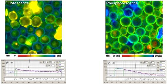
Fig. 36: Simultaneous FLIM and PLIM of yeast cells. Autofluorescence of the cells (left) and phosphorescence of a ruthenium compound (right)

Summary

Classic TCSPC records the waveform of a periodic optical signal by detecting single photons of the signal and building up of a photon distribution over the time in the signal period. The technique yields high sensitivity, near-ideal photon efficiency and extraordinarily high time resolution. With bh TCSPC devices an electrical IRF width of less than 3 ps FWHM is achieved. The system IRF with fast hybrid detectors is shorter than 20 ps FWHM; with superconduction nanowire detectors down to 4.4 ps FWHM have been achieved.

The disadvantage of the classic TCSPC method is that it is one-dimensional - it just delivers the waveform of the optical signal. In 1993, bh therefore introduced a multi-dimensional TCSPC technique. The technique is based on the idea that TCSPC records a photon distribution. Classic TCSPC records a photon distribution over the times of the photons in the excitation pulse period; multi-dimensional TCSPC records a photon distribution over the time in the excitation pulse period and one or more other parameters that can be associated to the individual photons. These may be the wavelength, the location in a sample where the photon came from, the time from a stimulation of the sample, or the time within the period of an additional modulation of the excitation light source. The result are techniques like multi-wavelength fluorescence decay recording, ultra-fast time series fluorescence decay recording, FLIM, multi-wavelength FLIM, ultra-fast time-series FLIM, spatial and temporal mosaic FLIM, and simultaneous FLIM / PLIM. The bh technique is open to the use of other parameters, such as temperature of the sample, oxygen partial pressure, or voltage applied to or measured at the sample. Thus, there may be possibilities which have even not been considered yet. Please see The bh TCSPC Handbook [16] for further suggestions and applications.

References

1. R.M. Ballew, J.N. Demas, An error analysis of the rapid lifetime determination method for the evaluation of single exponential decays, Anal. Chem. 61, 30 (1989)

2. Becker & Hickl GmbH, World Record in TCSPC Time Resolution: Combination of bh SPC-150NX with SCONTEL NbN Detector yields 17.8 ps FWHM. Application note, available on www.becker-hickl.com

3. Becker & Hickl GmbH, Sub-20ps IRF Width from Hybrid Detectors and MCP-PMTs. Application note, available on www.becker-hickl.com.

4. Becker & Hickl GmbH, SPC-QC-104 3/4 Channel TCSPC/FLIM Module, User Manual. Available on www.becker-hickl.com.

5. Becker & Hickl GmbH, DCS-120 Confocal and Multiphoton Scanning FLIM Systems, user handbook 9th ed. (2021). Available on www.becker-hickl.com

6. Becker & Hickl GmbH, Modular FLIM systems for Zeiss LSM 510 and LSM 710 family laser scanning microscopes. User handbook. Available on www.becker-hickl.com

7. Becker & Hickl GmbH, PML-16-C 16 and PML-16 GaAsP 16-channel channel TCSPC / Detectors, PML-SPEC and MW FLIM Multi-Wavelength detectors. User handbook (20016). Available on www.becker‑hickl.com

8. Becker & Hickl GmbH, bh - Abberior Combination Records STED FLIM at Megapixel Resolution. Application note, available on www.becker-hickl.com

9. Becker & Hickl GmbH, Simultaneous Phosphorescence and Fluorescence Lifetime Imaging by Multi-Dimensional TCSPC and Multi-Pulse Excitation. Application note, available on www.becker-hickl.com

10. Ultra-fast HPM Detectors Improve NAD(P)H FLIM. Application note, available on www.becker-hickl.com

11. Becker & Hickl GmbH, FLIM Systems for Laser Scanning Microscopes. Overview brochure, available on www.becker-hickl.com

12. W. Becker, Adva nced time-correlated single-photon counting techniques. Springer, Berlin, Heidelberg, New York, 2005

13. W. Becker, A. Bergmann, E. Haustein, Z. Petrasek, P. Schwille, C. Biskup, L. Kelbauskas, K. Benndorf, N. Klöcker, T. Anhut, I. Riemann, K. König, Fluorescence lifetime images and correlation spectra obtained by multi-dimensional TCSPC, Micr. Res. Tech. 69, 186-195 (2006)

14. W. Becker, A. Bergmann, C. Biskup, Multi-Spectral Fluorescence Lifetime Imaging by TCSPC. Micr. Res. Tech. 70, 403-409 (2007)

15. W. Becker, Fluorescence Lifetime Imaging - Techniques and Applications. J. Microsc. 247 (2) (2012)

16. W. Becker, The bh TCSPC handbook. 8th edition, Becker & Hickl GmbH (2019), available on www.becker-hickl.com

17. W. Becker, Introduction to Multi-Dimensional TCSPC. In W. Becker (ed.) Advanced time-correlated single photon counting applications. Springer, Berlin, Heidelberg, New York (2015)

18. W. Becker, V. Shcheslavskiy, H. Studier, TCSPC FLIM with Different Optical Scanning Techniques, in W. Becker (ed.) Advanced time-correlated single photon counting applications. Springer, Berlin, Heidelberg, New York (2015)

19. W. Becker, V. Shcheslavskiy, A. Rück, Simultaneous phosphorescence and fluorescence lifetime imaging by multi-dimensional TCSPC and multi-pulse excitation. In: R. I. Dmitriev (ed.), Multi-parameteric live cell microscopy of 3D tissue models. Springer (2017)

20. W. Becker, S. Frere, I. Slutsky, Recording Ca⁺⁺ Transients in Neurons by TCSPC FLIM. In:F.-J. Kao, G. Keiser, A. Gogoi, (eds.), Advanced optical methods of brain imaging. Springer (2019)

21. W. Becker, J. Breffke, B. Korzh, M. Shaw, Q.-Y. Zhao, K. Berggren, 4.4 ps IRF width of TCSPC with an NbN Superconducting Nanowire Single Photon Detector. Application note, available on www.becker-hickl.com

22. W. Becker, A. Bergmann, L. Braun, Metabolic Imaging with the DCS-120 Confocal FLIM System: Simultaneous FLIM of NAD(P)H and FAD, Application note, Becker & Hickl GmbH (2019)

23. Becker Wolfgang, Suarez-Ibarrola Rodrigo, Miernik Arkadiusz, Braun Lukas, Metabolic Imaging by Simultaneous FLIM of NAD(P)H and FAD. Current Directions in Biomedical Engineering 5(1), 1-3 (2019)

24. W. Becker, C. Junghans, A. Bergmann, Two-Photon FLIM of Mushroom Spores Reveals Ultra-Fast Decay Component. Application note, available on www.becker-hickl.com.

25. W. Becker, T. Saeb-Gilani, C. Junghans, Two-Photon FLIM of Pollen Grains Reveals Ultra-Fast Decay Component. Application note, available on www.becker-hickl.com

26. Wolfgang Becker, V. Shcheslavskiy, Axel Bergmann, FLIM at a Time-Channel Width of 300 Femtoseconds. Application note, available on www.becker-hickl.com.

27. W. Becker, V. Shcheslavskiy, V. Elagin Ultra-Fast Fluorescence Decay in Malignant Melanoma. Application note, available on www.becker-hickl.com.

28. W. Becker, A. Bergmann, L. Sauer, Shifted-Component Model Improves FLIO Data Analysis. Application note, Becker & Hickl GmbH (2019)

29. L. M. Bollinger, G. E. Thomas, Measurement of the time dependence of scintillation intensity by a delayed coincidence method. Rev. .Sci. Instrum. 32, 1044-1050 (1961)

30. D. Chorvat, A. Chorvatova, Multi-wavelength fluorescence lifetime spectroscopy: a new approach to the study of endogenous fluorescence in living cells and tissues. Laser Phys. Lett. 6 175-193 (2009)

31. S. Cova, M. Bertolaccini, C. Bussolati, The measurement of luminescence waveforms by single-photon techniques, Phys. Stat. Sol. 18, 11-61 (1973)

32. Dysli, C., Wolf, S., Berezin, M.Y., Sauer, L., Hammer, M., Zinkernagel, M.S., Fluorescence lifetime imaging ophthalmoscopy, Progress in Retinal and Eye Research (2017), doi: 10.1016/j.preteyeres.2017.06.005

33. S. Frere, I. Slutsky, Calcium imaging using Transient Fluorescence-Lifetime Imaging by Line-Scanning TCSPC. In: W. Becker (ed.) Advanced time-correlated single photon counting applications. Springer, Berlin, Heidelberg, New York (2015)

34. J. Jenkins, R. I. Dmitriev, D. B. Papkovsky, Imaging Cell and Tissue O₂ by TCSPC-PLIM. In: W. Becker (ed.) Advanced time-correlated single photon counting applications. Springer, Berlin, Heidelberg, New York (2015)

35. S. Kalinina, V. Shcheslavskiy, W. Becker, J. Breymayer, P. Schäfer, A. Rück, Correlative NAD(P)H-FLIM and oxygen sensing-PLIM for metabolic mapping. J. Biophotonics 9(8):800-811 (2016)

36. S. Kinoshita, T. Kushida, Subnanosecond fluorescence-lifetime measuring system using single photon counting method with mode-locked laser excitation, Rev. Sci. Instrum. 52, 572-575 (1981)

37. M. Köllner, J. Wolfrum, How many photons are necessary for fluorescence-lifetime measurements?, Phys. Chem. Lett. 200, 199-204 (1992)

38. H. Kurokawa, H. Ito, M. Inoue, K. Tabata, Y. Sato, K. Yamagata, S. Kizaka-Kondoh, T. Kadonosono, S. Yano, M. Inoue & T. Kamachi, High resolution imaging of intracellular oxygen concentration by phosphorescence lifetime, Scientific Reports 5, 1-13 (2015)

39. C. Lewis, W.R. Ware, The Measurement of Short-Lived Fluorescence Decay Using the Single Photon Counting Method, Rev. Sci. Instrum. 44, 107-114 (1973)

40. B. Leskovar, C.C. Lo, Photon counting system for subnanosecond fluorescence lifetime measurements, Rev. Sci. Instrum. 47, 1113-1121 (1976)

41. A. Marcek Chorvatova, Time-Resolved Spectroscopy of NAD(P)H in Live Cardiac Myocytes. In: W. Becker (ed.) Advanced time-correlated single photon counting applications. Springer, Berlin, Heidelberg, New York (2015)

42. S. Pallikkuth, D. J. Blackwell, Z. Hu, Z. Hou, D. T. Zieman, B. Svensson, D. D. Thomas, S. L. Robia, Phosphorylated Phospholamban Stabilizes a Compact Conformation of the Cardiac Calcium-ATPase. Biophys. J. 105, 18121821 (2013)

43. A. Periasamy, N. Mazumder, Y. Sun, K. G. Christopher, R. N. Day, FRET Microscopy: Basics, Issues and Advantages of FLIM-FRET Imaging. In: W. Becker (ed.) Advanced time-correlated single photon counting applications. Springer, Berlin, Heidelberg, New York (2015)

44. D.V. OConnor, D. Phillips, Time-correlated single photon counting, Academic Press, London (1984)

45. R. Rigler, E.S. Elson (eds), Fluorescence Correlation Spectroscopy, Springer Verlag Berlin, Heidelberg, New York (2001)

46. A. Rück, Ch. Hülshoff, I. Kinzler, W. Becker, R. Steiner, SLIM: A New Method for Molecular Imaging. Micr. Res. Tech. 70, 403-409 (2007)

47. V. I. Shcheslavskiy, M. V. Shirmanova, V. V. Dudenkova, K. A. Lukyanov, A. I. Gavrina, A. V. Shumilova, E. Zagaynova, W. Becker, Fluorescence time-resolved macroimaging. Opt. Lett. 43, No. 13, 3152-5155 (2018)

48. V. I. Shcheslavskiy, M. V. Shirmanova, A. Jelzow, W. Becker, Multiparametric Time-Correlated Single Photon Counting Luminescence Microscopy. Biochemistry (Moscow), 84, Suppl. 1, pp. S51-S68 (2019)

49. R. Suarez-Ibarrola, L. Braun, P. F. Pohlmann, W. Becker, A. Bergmann, C. Gratzke, A. Miernik, K. Wilhelm, Metabolic Imaging of Urothelial Carcinoma by Simultaneous Autofluorescence Lifetime Imaging (FLIM) of NAD(P)H and FAD. Clinical Genitourinary Cancer (2020)

50. R. Schuyler, I. Isenberg, A Monophoton Fluorometer with Energy Discrimination, Rev. Sci. Instrum. 42 813-817 (1971)

51. D. Schweitzer, M. Hammer, Fluorescence Lifetime Imaging in Ophthalmology. In: W. Becker (ed.) Advanced time-correlated single photon counting applications. Springer, Berlin, Heidelberg, New York (2015)

52. D. Singh, H. Sielaff, M. Börsch, G. Grüber, Conformational dynamics of the rotary subunit F in the A₃B₃DF complex of Methanosarcina mazei Gö1 A-ATP synthase monitored by single-molecule FRET.FEBS Letters 591, 854-862 (2017)

53. J. Yguerabide, Nanosecond fluorescence spectroscopy of macromolecules, Meth. Enzymol. 26, 498-578 (1972)