The bh FLIM systems for the Zeiss LSM 710 /780 / 880 / 980 family laser scanning microscopes are based on bh’s Multi-Dimensional TCSPC technique and 64 bit Megapixel technology. The systems feature single-photon sensitivity, excellent spatial and temporal resolution, multi-exponential decay analysis, and short acquisition time. The systems are available both for confocal and for multiphoton versions of the Zeiss LSMs. The recording functions include basic FLIM recording, dual-channel FLIM, excitation-wavelength-multiplexed FLIM, Z stack FLIM, time-series FLIM, spatial and temporal mosaic FLIM, fluorescence lifetime-transient scanning (FLITS), and phosphorescence lifetime imaging (PLIM). Multi-spectral FLIM is available by adding a special detector to the system. Unlike other systems, the bh FLIM systems are true molecular imaging systems. They use the fluorescence lifetime not only as a contrast parameter but as an indicator of the molecular state of the sample. This becomes possible by recording the complex multi-exponential decay behaviour in the individual pixels and analysing the data with advanced data analysis procedures based on a combination of MLE-based time-domain analysis, phasor analysis, and image segmentation functions. This brochure gives an overview of the recording functions of the systems, the data analysis, and the application to FRET measurements, autofluorescence FLIM of tissue, metabolic imaging, time-resolved recording of fast physiological processes, and plant physiology. For complete information please see handbook of the bh FLIM systems for the Zeiss LSM series microscopes and addendum for LSM 980 microscopes.
FLIM Systems for Zeiss LSM 710 / 780 / 880 / 980
Laser Scanning Microscopes
An Overview
Abstract: The FLIM systems for the Zeiss LSM 710 /780 / 880 / 980 family laser scanning microscopes are based on bhs Multi-Dimensional TCSPC technique and 64 bit Megapixel technology [24, 31]. The systems feature single-photon sensitivity, excellent spatial and temporal resolution, multi-exponential decay analysis, and short acquisition time. The systems are available both for confocal and for multiphoton versions of the Zeiss LSMs. The recording functions include basic FLIM recording, dual-channel FLIM, excitation-wavelength-multiplexed FLIM, Z stack FLIM, time-series FLIM, spatial and temporal mosaic FLIM, fluorescence lifetime-transient scanning (FLITS), and phosphorescence lifetime imaging (PLIM). Multi-spectral FLIM is available by adding a special detector to the system. Unlike other systems, the bh FLIM systems are true molecular imaging systems. They use the fluorescence lifetime not only as a contrast parameter but as an indicator of the molecular state of the sample. This becomes possible by recording the complex multi-exponential decay behaviour in the individual pixels and analysing the data with advanced data analysis based on a combination of MLE-based time-domain analysis, phasor analysis, and image segmentation functions. This brochure gives an overview of the recording functions of the systems, the data analysis, and the application to FRET measurements, autofluorescence FLIM of tissue, metabolic imaging, and time-resolved recording of fast physiological processes. For complete information please see The bh TCSPC Handbook [31], Handbook of the bh FLIM systems for the Zeiss LSM series microscopes [2], and addendum for LSM 980 microscopes [3].
Introduction
Becker & Hickl introduced their multi-dimensional TCSPC technique in 1993. Fluorescence lifetime imaging started in 1996 with applications in ophthalmology [90]. The first FLIM module for laser scanning microscopes was introduced in 1998, bh FLIM systems for the Zeiss LSM laser scanning microscopes are available since 2000 [21]. Since then, several new generations of LSM family laser scanning microscopes, and several generations of bh FLIM modules have been introduced. As a result, a wide variety of bh FLIM systems and of FLIM system configurations are in use [24, 31]. The excitation light source can be the Ti:Sapphire laser of a multiphoton microscope, a picosecond diode laser attached to or integrated in the microscope, or a visible-range tuneable solid state laser. The fluorescence light may be detected via a confocal port of the scan head or via a non-descanned port of a multiphoton microscope. Signals may be detected by one detector, simultaneously by two, three, or four detectors, or by the 16 channels of a bh multi-wavelength detector.
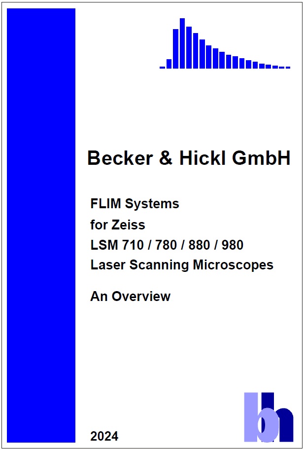
All bh FLIM systems are using highly efficient GaAsP hybrid detectors, combining extremely high efficiency with large active area, high counting speed, short acquisition time, high time-resolution, and low background [31]. Moreover, the systems are using 64-bit data acquisition software [7], which enables the FLIM system to record data at unprecedented pixel numbers and numbers of time channels. FLIM data analysis is performed by bh's legendary SPCImage NG software [4, 32]. SPCImage NG combines time-domain [32] and phasor [57] analysis, uses an MLE algorithm [32] to fit the data, and runs the calculation on a GPU, resulting in data processing times of no more than a few seconds. These features make the bh FLIM systems superior to other systems even in entry-level FLIM applications. An example of a high-resolution FLIM image is shown in Fig. 1.
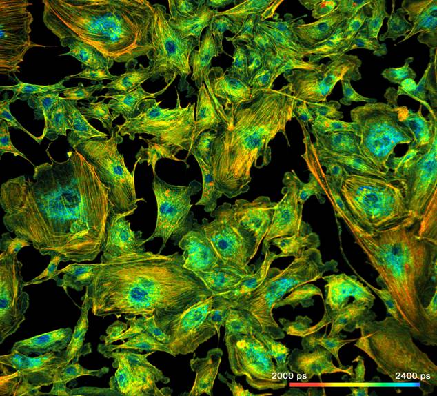
Fig. 1: High-resolution FLIM image of BPAE cells, recorded by a bh TCSPC FLIM system.
Most importantly, the bh FLIM systems are based on a new understanding of FLIM in general. FLIM is no longer considered simply a way of adding lifetime contrast to a microscopy image. It is considered a technique of molecular imaging, i.e. of recording and visualising molecular parameters and molecular processes in biological systems. Following this idea, the FLIM systems are designed to observe several parameters of biological system simultaneously, and in their mutual dependence. This is supported by advanced FLIM functions, like multi-channel operation, excitation-wavelength-multiplexing, time-series FLIM, Z stack FLIM, spatial and temporal Mosaic FLIM, multi-wavelength FLIM, simultaneous fluorescence and phosphorescence lifetime imaging (FLIM/PLIM), fluorescence lifetime-transient scanning (FLITS), and combinations of these techniques [31]. An overview on the functions of the bh FLIM systems is given in Fig. 2. For a detailed description please see [2] and [3]. Please see also 'Application Notes' on www.becker-hickl.com. Moreover, we recommend [24, 31, 38] as supporting literature.
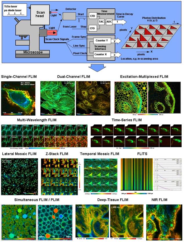
Fig. 2: Overview on bh FLIM functions
Optical Architecture of the LSM 710 / 780 / 880 / 980 FLIM Systems
All bh TCSPC FLIM systems have in common that the sample is excited by a pulsed laser of high repetition rate, scanned at high pixel rate by the optical scanner of the microscope, and that the fluorescence light is detected by one or several fast photon counting detectors connected to the microscope. The FLIM data are recorded by building up a photon distribution over the times of the photons in the laser pulse period and the positions of the laser beam in the moment of the photon detection [24]. Typical FLIM configurations for the LSM 710/780/880/980 family microscopes are shown in Fig. 3 through Fig. 7.
Fig. 3 shows FLIM configurations for inverted microscopes. The configuration on the left uses multiphoton excitation by a femtosecond titanium-sapphire laser for excitation. The fluorescence light is detected via a non-descanned detection (NDD) beam path. Typically, the light is split in two spectral components by a Zeiss 'T Adapter', and detected by two parallel detectors and TCSPC channels.
The configuration shown on the right uses confocal detection. The sample is excited by one-photon excitation. The excitation source can either be a single bh BDL-SMC or BDL-SMC laser or a bh 'Laser Hub' with four separate BDS-SMC lasers. The fluorescence light is detected back through the confocal beam path of the scanner and sent out of the scan head via an optical port. It is split into two spectral channels by a bh beamsplitter module and fed into two FLIM detectors. The single-photon pulses from the detectors are recorded by two separate TCSPC channels of the FLIM system.
Fig. 3: LSM 710/780 family FLIM systems, inverted microscopes. Left: Multiphoton-excitation FLIM with non-descanned detection. Right: One-photon FLIM with confocal detection.
The detectors and detector assemblies for the confocal port are compatible with those for the NDD port. That means the detectors can be moved between the two port. It is also possible to attach detectors to the both ports permanently. The desired pair of detectors can then be selected in the SPCM data acquisition software.
Fig. 4 shows FLIM at an LSM 710/780/880/980 in the upright version. The configuration on the left uses multiphoton excitation and non-descanned detection, the configuration on the right uses one-photon excitation and confocal detection.
Fig. 4: LSM 710/780/880/980 family FLIM systems, upright microscopes. Left: Multiphoton-excitation FLIM with non-descanned detection. Right: One-photon excitation FLIM with confocal detection.
Multiphoton and the one-photon FLIM configurations for the LSM 880 and LSM 980 with Airy-Scan detectors are shown in Fig. 5, left and right. For the multiphoton system there is no difference to the standard system. The Airy-Scan detector rests at the confocal port and does not interfere with the FLIM detectors at the NDD port. In the one-photon FLIM system the FLIM detectors are connected to a beam switch between the scan head and the Zeiss Airy-Scan detector, see Fig. 5, right.
Fig. 5: LSM 880 / 980 FLIM systems, inverted microscopes. Left: Multiphoton-excitation FLIM with non-descanned detection. Right: One-photon excitation FLIM with confocal detection.
Standard bh FLIM systems for the LSM 710, 780, 880, and 980 use the bh HPM‑100-40 or -06 hybrid detectors [31, 27]. The systems are also available with the NIR versions of the HPM‑100 detectors [8, 9, 37]. LSMs which have a Zeiss BIG-2 detector [50] can use this detector for FLIM [10, 31]. The BIG‑2 is not as fast as the hybrid detectors, but it is well suitable for standard FLIM applications. Systems with the BIG-2 detector are extremely easy to be set up. In fact, BIG-2 multiphoton systems require nothing than the TCSPC electronics and a few cable connections. One-photon ('Confocals') systems need a bh ps diode laser or a bh Laser Hub connected to one of the laser inputs of the LSM. The basic setup of the bh FLIM systems with the BIG-2 detector is shown in Fig. 6.
Fig. 6: FLIM systems using the Zeiss BIG-2 detector. Left: Multiphoton system. Right: Confocal system
The bh FLIM systems for Zeiss LSMs work also with the bh MW-FLIM GaAsP multi-spectral FLIM detectors [31]. With these detectors, the FLIM systems record in 16 spectral channels simultaneously. The optical configuration for multiphoton multi-wavelength FLIM is shown in Fig. 7. The light is collected from an NDD port by a fibre bundle. The light is dispersed spectrally, and detected by a bh PML-16 GaAsP (16-channel) PMT module. Similarly, the multi-wavelength FLIM detector assembly can be attached to the confocal port of the scan head.

Fig. 7: Multi-wavelength FLIM
Principle of Data Acquisition
Multi-Dimensional TCSPC
The bh FLIM systems use a combination of bhs multidimensional time-correlated single-photon counting process with confocal or multiphoton laser scanning [24, 31, 39, 40]. The principle is shown in Fig. 8. The laser scanning microscope scans the sample with a focused beam of a high-repetition-rate pulsed laser. Depending on the laser used, the fluorescence in the sample can either be excited by one-photon or by multiphoton excitation. The FLIM detector is attached either to a confocal or non-descanned port of the laser scanning microscope [2, 21, 22, 23, 29, 31]. For every detected photon the detector sends an electrical pulse into the TCSPC module. Moreover, the TCSPC module receives scan clock signals (pixel, line, and frame clock) from the scanning unit of the microscope.
Fig. 8: Multidimensional TCSPC architecture for FLIM
For each photon pulse from the detector, the TCSPC module determines the time within the laser pulse sequence (i.e. in the fluorescence decay) and the location within the scanning area, x and y. The photon times, t, and the spatial coordinates, x and y, are used to address a memory in which the detection events are accumulated. Thus, in the memory the distribution of the photon density over x, y, and t builds up. The result is a data array representing the pixel array of the scan, with every pixel containing a large number of time channels with photon numbers for consecutive times after the excitation pulse. In other words, the result is an image that contains a fluorescence decay curve in each pixel [23, 24]. An example is shown in Fig. 9.
Standard bh FLIM systems have two parallel channels of the architecture shown in Fig. 8. The systems are therefore able to simultaneously record images in two spectral channels. Because the channels are parallel the systems deliver high throughput rates. Another advantage is that the channels are independent. If one channel overloads the other one still delivers correct data. Please see [2] and [31] for details.
Fast Scanning Capability
It should be explicitly noted that FLIM by multi-dimensional TCSPC does not require that the scanner stays in one pixel until enough photons for a full fluorescence decay curve have been acquired. It is only necessary that the total pixel time, over a large number of subsequent frames, is large enough to record a reasonable number of photons per pixel. Thus, TCSPC FLIM works even at the highest scan rates available in laser scanning microscopes. At the pixel rates used in practice, the recording process is more or less random: A photon is just stored in a memory location according to its time in the fluorescence decay, its detector channel number, and the location of the laser spot in the sample in the moment of detection.
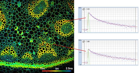
Fig. 9: FLIM image of a Convallaria Sample, 2048x2048 pixels. Every pixel contains a fluorescence decay curve resolved in a large number of time channels.
Time Resolution
bh FLIM systems are unsurpassed in time resolution. With the new SPC-180NX TCSPC modules the systems reach unprecedented timing stability and time resolution. The electrical time resolution is better than 3 ps (FWHM!), the timing stability better than 0.5 ps (RMS) [31, 36] (Fig. 10, left and middle). The time channel width (often incorrectly termed 'time resolution') can be as short as 200 femtoseconds. With the new ultra-fast HPM‑100-06 detectors, the instrument-response function for multiphoton systems is <20 ps (FWHM), see Fig. 10, right. Timing performance on this level is entirely beyond of the reach of any other FLIM system. With their fast detectors and negligible timing jitter of the electronics, the systems accurately record ultra-fast fluorescence-decay components which previously were unknown to even exist [44, 45, 46, 47]. Moreover, the time resolution does not degrade over extended acquisition times. Extremely weak signals or signals from extremely fragile samples can therefore be recorded successfully. The high stability in combination with the automatic IRF-calibration function of SPCImage makes it unnecessary to re-calibrate the system by repeated recording of the instrument-response function (IRF). This is a significant advantage for practical use.
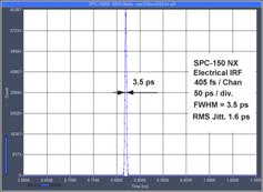
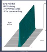
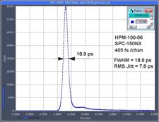
Fig. 10, left to right: Electrical IRF of SPC-180NX, IRF stability over 100 s, IRF of multiphoton system with HPM-100-06
Multi-exponential-Decay Capability
Importantly, the bh FLIM technique delivers the complete temporal profile of the decay functions in the pixels, not only an average 'fluorescence lifetime' [24, 38]. This is extremely important for biological applications, where the primary information often is in the composition of the multi-exponential decay rather than in a simple lifetime.
Photon Efficiency for Single and Multiexponential Decay
In combination with bh's SPCImage NG data analysis software, the bh FLIM systems feature near-ideal photon efficiency. That means the number of photons needed to reach a given lifetime accuracy is close to the theoretical minimum [6]. Due to the high time resolution and the large number of time channels per pixel excellent photon efficiency is not only achieved for single-exponential 'lifetimes' but also for the parameters of multi-exponential decay functions. The ability to derive multi-exponential decay parameters from the FLIM data is the basis of molecular imaging and other high-end FLIM applications.
Acquisition Time
Near-ideal photon efficiency means that the system reaches minimum acquisition time for a desired decay-parameter accuracy at a given photon rate. That means the bh FLIM systems reach minimum acquisition time under conditions where the emission rate is limited by the photostability of the sample [6, 31]. This is the case in the majority of molecular imaging applications.
Multi-Parameter Recording
The most intriguing feature of the bh FLIM technique is the multi-dimensional nature of the recording process. bh FLIM systems are able to record at several excitation wavelengths simultaneously, record dynamic processes in live samples down to the millisecond range, record FLIM and PLIM simultaneously, or record multi-spectral FLIM images. With these capabilities, bh FLIM systems are ideal molecular-imaging systems, able to observe several parameters of biological system simultaneously and in their mutual dependence [31].
FCS and Single-Molecule Capabilities
The TCSPC module can also process the photon data to obtain fluorescence-correlation data (FCS) data [31, 25], photon counting histograms (PCH) or photon-counting-lifetime histograms. Moreover the parameter-tagged single photon data can be stored in a file for off-line processing by single-molecule spectroscopy techniques.
TCSPC Modules
Different generations if the bh FLIM systems contain different TCSPC / FLIM modules. Early bh FLIM systems used SPC-830 or SPC-150 modules. From 2016 on SPC150 N and SPC-150 NX modules were used. The SPC-150 N, and, especially, the SPC-150 NX achieve higher time resolution in combination with ultra-fast hybrid detectors and femtosecond lasers. Recent systems use either the SPC‑180 NX or the SPC-QC-104. The SPC-180 NX delivers maximum time resolution with fast detectors and lasers, the SPC-QC has lower time resolution but can record at extremely high count rates. Still, the instrument response (IRF) of the SPC‑QC 104 is faster than the pulse width of diode lasers and faster than the transit-time spread of most detectors, see Fig. 12. Hence there is little difference in resolution for confocal systems with diode lasers. For NLO systems with femtosecond lasers, however, it can be the difference between easily detecting a fast decay component and missing it.
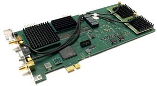
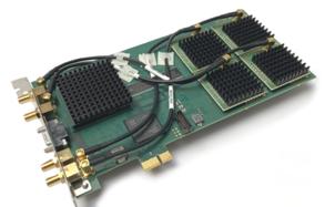
Fig. 11: SPC-180 NX (left) and SPC-QC-104 (right)
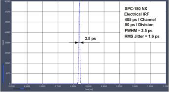
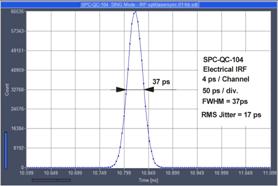
Fig. 12: Electrical IRF for SPC-180 NX (left) and SPC-QC 104
Lasers
Confocal FLIM
bh FLIM systems for the LSM 710, 780, and 880 confocal microscopes had one or two ps diode lasers. These were integrated in the hardware and software of the Zeiss LSM systems. With just two laser wavelengths and limited control over the laser function, these systems were limited both in excitation wavelength and recording functions. The LSM 980 confocal FLIM systems are coming with four ps diode lasers of different wavelength [3]. The lasers are contained in the LHB-104 Laser Hub [5], shown in Fig. 13. The lasers are coupled into the LSM 980 scan head via a single-mode fibre by a standard Zeiss / Lasos fibre coupler. The lasers can be switched on an off on demand, multiplexed in time for excitation-wavelength multiplexed FLIM, or on/off modulated for simultaneous FLIM / PLIM.
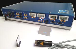
Fig. 13: LBH-104 Laser Hub. Output of four wavelengths via single fibre with Zeiss / Lasos coupler, demonstrated by reflection off an optical grating.
Multiphoton FLIM
The bh FLIM systems work both with the confocal versions and with the multiphoton versions of the Zeiss LSMs. The excitation source in multiphoton systems is normally a Ti:Sa laser. The FLIM systems are perfectly compatible with these lasers [2]. In principle, they also work with femtosecond fibre lasers [16], should one of these be used in combination with a Zeiss LSM.
Detectors
The bh FLIM systems for the Zeiss LSMs are using the bh HPM-100 hybrid detectors [27]. The advantage of these detectors is that they have a fast and clean TCSPC response (Instrument-response function, IRF), and that they have no afterpulsing. The fast IRF and the absence of afterpulsing background have the effect that FLIM data analysis works close to the theoretical limit of photon efficiency [6]. Two versions of the HPM-100 are used for FLIM. The HPM-100-40 is used in applications which require highest sensitivity [27], the HPM-100-06 in applications which require highest time resolution [15]. Detectors and detector assemblies are compatible both with the BIG port of confocal microscopes and with the NDD ports of multiphoton microscopes. The detectors and detector assemblies are fully integrated in the laser-safety loop of the LSM systems.
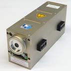
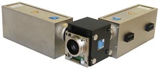
Fig. 14: HPM-100 hybrid detector and dual-detector assembly with adapter to the optical ports of the Zeiss LSM systems
The bh FLIM systems also work with the Zeiss GaAsP BIG-2 detectors [10]. The time resolution with these detectors does not reach the resolution of the HPM detectors, but using them has the advantage that no additional hardware has to be attached to the microscope. Additionally, there is the bh MW FLIM detector for recording multi-spectral FLIM data. Also this detector is available with a highly efficient GaAsP cathode [31].
SPCM Data Acquisition Software
The bh TCSPC FLIM Systems come with the Multi SPC Software, SPCM, a software package that allows the user to operate up to four bh TCSPC / FLIM modules. SPCM runs the data acquisition in the various operation modes of the SPC modules while controlling peripheral devices, such as detectors and lasers. Operation modes are available for almost any conceivable TCSPC application, such as fluorescence and phosphorescence decay recording, multi-wavelength decay recording, laser-wavelength multiplexing, recording of time series, FCS and photon counting histograms, single-, dual, or quadruple-channel FLIM, multi-wavelength FLIM, Mosaic FLIM, time-series FLIM, Z stack FLIM, and simultaneous FLIM / PLIM. Current bh SPCM data acquisition software includes fast online-FLIM display and online display of decay curves in selectable regions or points of interest, see Fig. 22, page 19. Moreover, recent SPCM versions have been upgraded with extended multi-threading functions, avoiding bus saturation even at the highest count rates and when computation-intensive functions like online FLIM and ROI-curve display are used [31].
A typical SPCM user interface is shown in Fig. 15. It shows lifetime images of pig skin, recorded in different wavelength intervals in two parallel channels of the FLIM system. The left image shows NADH and SHG, the right image FAD.
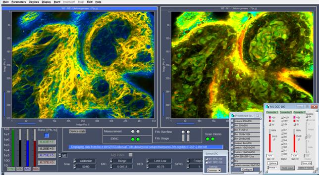
Fig. 15: User Interface of SPCM data acquisition software. Pig skin, 2p excitation, two wavelength channels, online lifetime display, predefined setups for frequently used operation modes, detector control.
Fig. 16 shows a user interface configuration for simultaneous FLIM / PLIM. From left to right, the display windows show an NADH lifetime image, an FAD lifetime image, and an intensity image of the phosphorescence of a Ruthenium dye.
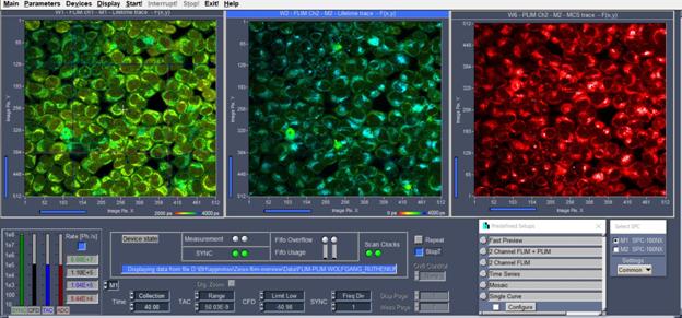
Fig. 16: SPCM Data Acquisition Software, simultaneous FLIM / PLIM. Left to right: NADH image, FAD image, phosphorescence image.
SPCM Integration in Zeiss ZEN Software
bh / Zeiss FLIM systems are available with bh's new integrated SPCConnect software. It combines bh SPCM software, bh SPCIMage NG software, and Zeiss ZEN software by a TCP (Transmission Control Protocol). That means SPCM and SPCImage NG are running in the frame of ZEN, with all components freely exchanging commands, system parameters, and data. Compared to an integration on the DLL level TCP integration has the advantage that, in addition to basic FLIM, functions like Z-stack recording, time-series recording, fast triggered accumulation, FLITS, and simultaneous FLIM / PLIM are included. Examples of the integrated ZEN / SPCM user interface are shown in Fig. 17 and Fig. 18.
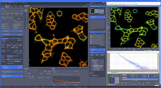
Fig. 17: Integration of bh SPCM FLIM data acquisition and control software in Zeiss ZEN software
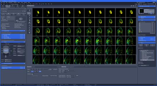
Fig. 18: Z stack recording with integrated ZEN / SPCM software
SPCImage NG Data Analysis Software
The LSM 710 /780 / 880 / 980 FLIM systems use bhs SPCImage NG next generation data analysis software [4, 32]. SPCImage NG is a combination of time-domain [32] and phasor [57] analysis. It uses maximum-likelihood estimation (MLE) to calculate the FLIM images, resulting in superior photon efficiency of multi-exponential decay analysis. Image segmentation via the phasor plot allows decay parameters to be precisely determined even in data of low photon number. Calculations are running on a GPU (graphics-processor unit). By GPU processing, calculation times are reduced from formerly more than 10 minutes to a few seconds. Another novel feature is advanced modelling of the system IRF [32]. In combination with the extraordinary timing stability of the bh FLIM system, IRF modelling makes the recording of an IRF unnecessary. Please see [4] or [32] for details. Examples of data analysis with SPCImage are shown in Fig. 19 and Fig. 20.
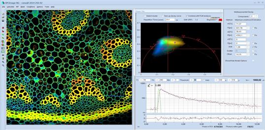
Fig. 19: SPCImage NG Data analysis software. FLIM image (left), phasor plot (upper right), decay curve at cursor position (lower right).
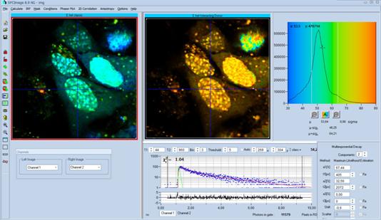
Fig. 20: SPCImage NG, FRET analysis. Classic FET efficiency (left) and FRET efficiency of interacting donor fraction (right). Both are derived from a single lifetime image of the donor [34].
General Features of the bh FLIM Technique
Megapixel FLIM Images
With bhs megapixel technology, pixel numbers can be increased up to 2048 x 2048 while maintaining a temporal resolution of 256 time channels. Alternatively, the number of time channels can be increased up to 1024 for images of 1024x1024 pixels, and up to 4096 for images of 512x512 pixels or less. Thus, the useful pixel resolution is rather limited by the optical resolution and the maximum field of view of the microscope lens than by the capabilities of the bh FLIM system.
Fig. 21 shows a FLIM image of a BPAE sample recorded at a resolution of 1024 x 1024 pixels. The image on the left shows the entire area of the scan. The image on the right is a digital zoom into the data shown left.
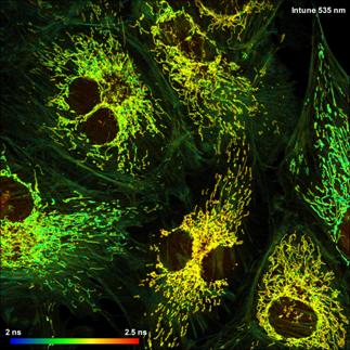
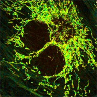
Fig. 21: Left: Image recorded with 1024 x 1024 pixels. Right: Digital zoom into the data of Fig. 21, showing the two cells on the upper left.
Large pixel numbers are important especially for tissue imaging. They are also useful in cases when a large number of cells have to be investigated and the FLIM results to be compared. Megapixel FLIM records images of many cells simultaneously, and under identical environment conditions. Moreover, the data are analysed in a single analysis run, with identical IRFs and fit parameters. The results are therefore exactly comparable for all cells in the image area.
Online Display of FLIM Images and Decay Curves
SPCM data acquisition software is able to display lifetime images and decay curves in selected spots or regions of interest of the images. This helps the user evaluate the progress of the recording, and, if necessary, make corrections in the laser power, the filter settings, or select a different imaging area or a different focal plane. Please see Fig. 22.
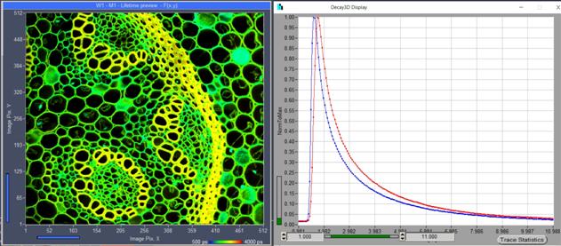
Fig. 22: Online display of lifetime images (left) and online display of decay curves in selectable regions of interest (right)
Ultra-High Efficiency
With its hybrid detectors, its multi-dimensional TCSPC process, its high time-resolution and its highly efficient data analysis the bh FLIM system delivers lifetime images at near-ideal photon efficiency [6]. Typical applications are precision FLIM data from weakly fluorescent samples, label-free imaging, and metabolic imaging by NADH or FAD FLIM [31, 43, 49, 53, 67]. An example is shown in Fig. 23.
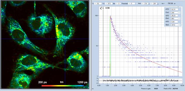
Fig. 23: Two-photon autofluorescence FLIM of single cells. NADH image, excitation 750 nm, detection from 440 to 480 nm, triple-exponential fit with SPCIMage NG.
Two fully parallel TCSPC FLIM Channels
Standard bh FLIM systems record in two wavelength intervals simultaneously. The signals are detected by separate detectors and processed by separate TCSPC modules [31]. There is no intensity or lifetime crosstalk. Even if one channel overloads the other channel is still able to produce correct data.
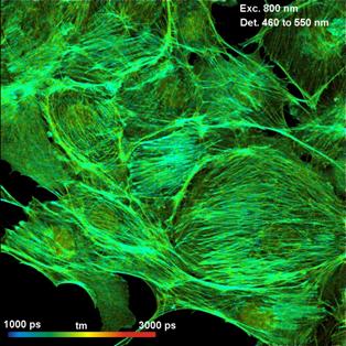
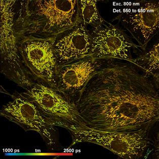
Fig. 24: Dual-channel detection. BPAE cells stained with Alexa 488 phalloidin and Mito Tracker Red. Left: 460 nm to 550 nm. Right: 550 nm to 650 nm.
Multiphoton NDD FLIM: Clean Images from Deep Tissue Layers
The bh Multiphoton FLIM systems use the non-descanned detection (NDD) path of the LSM 710/780/880/980 NLO family microscopes. With non-descanned detection, fluorescence photons scattered on the way out of the sample are detected far more efficiently than in a confocal system. The result is that clear images are obtained from deep tissue layers. An example is shown in Fig. 25. The images show a pig skin sample exited by two-photon excitation at 800 nm. The left image shows the wavelength channel below 480 nm. This channel contains both fluorescence and SHG signals. The SHG fraction of the signal has been extracted from the FLIM data and displayed by colour. The right image is from the channel >480 nm. It contains only fluorescence, the colour corresponds to the amplitude-weighted mean lifetime of the multi-exponential decay functions.
An often neglected advantage of multiphoton FLIM is that it can reach fluorophores with excitation wavelengths the ultraviolet region. It has been shown that Tryptophane can be reached by three-photon excitation [1]. Another important example is NADH, which, by one-photon excitation, requires 350 to 370 nm. This is, at least, an inconvenient wavelength, where scanner optics and microscope lenses do not perform well. With two-photon excitation, the laser wavelength is in the range of 750 to 780 nm, which is easy to handle both for the scanner optics and the microscope lens. For examples, please see Fig. 23 and Fig. 26.
An additional benefit of a multiphoton FLIM system is the very fast IRF. There is virtually no contribution to the IRF from the laser pulse itself, so that the effective IRF width is that of the detector itself. Please see next paragraph.
Fig. 25: Two-photon FLIM of pig skin. LSM 710 NLO, HPM‑100‑40, NDD. Left: Wavelength channel <480nm, colour shows percentage of SHG. Right: Wavelength channel >480nm, colour shows amplitude-weighted mean lifetime.
FLIM with Ultra-Fast Detectors
The instrument-response function of a multiphoton FLIM system with HPM-100-06 detectors has a full-width at half maximum (FWHM) of less than 20 ps [15, 36]. The fast response greatly improves the accuracy at which fast decay components can be extracted from a multi-exponential decay. Applications are mainly in the field of metabolic FLIM, which requires separation of the decay components of bound and unbound NADH, and in the range of FRET, which requires the separation of interacting and non-interacting donor components. An NADH FLIM image recorded with an ultra-fast FLIM system on a Zeiss LSM 880 NLO is shown in Fig. 25. Images of the images of the amplitude ratio, a1/a2 (unbound/bound ratio), and of the fast (t1, unbound NADH) and the slow decay component (t2, bound NADH) are shown in Fig. 27.
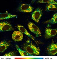
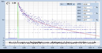
Fig. 26: Left: NADH Lifetime image, amplitude-weighted lifetime of double-exponential fit. Right: Decay curve in selected spot, 9x9 pixel area. FLIM data format 512x512 pixels, 1024 time channels. The IRF width is 19 ps, the time-channel width 10ps.
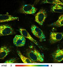
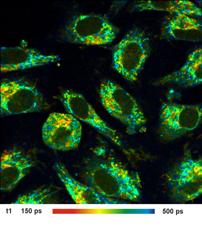
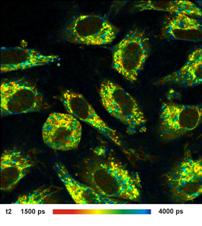
Fig. 27: Left to right: Images of the amplitude ratio, a1/a2 (unbound/bound ratio), and of the fast (t1, unbound NADH) and the slow decay component (t2, bound NADH). FLIM data format 512x512 pixels, 1024 time channels. Time-channel width 10ps.
Fig. 28 shows mushroom spores of Cortinarius mucosus. An image of the amplitude-weighted lifetime, tm, is shown on the left, a decay curve on the right. tm is in the range from 20 to 40 ps, the lifetime of the fast component, t1, in the range from 10 to 20 ps. No other FLIM system is able to show such fast decay processes directly.
Ultra-fast decays in biological material are more frequent than commonly believed. Similarly fast decay components were found in other mushroom spores [44], in pollen grains [45], in natural carotenoids [46], in human hair [47] and in malignant melanoma [48]. Ultra-fast fluorescence decay times should therefore no longer be put aside as a peculiarity but seriously considered as a potential source of biological information.
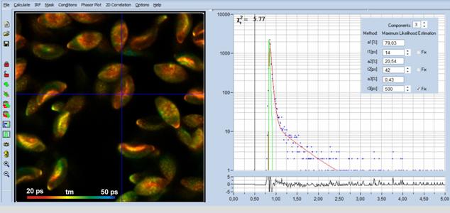
Fig. 28: FLIM of Mushroom spores, Cortinarius mucosus, 2p excitation at 760 nm. Image of the amplitude-weighted lifetime, tm, and decay curve at cursor position. tm is in the range from 20 to 40 ps, t1 is in the range from 10 to 20 ps.
FLIM with Tuneable Excitation Wavelength
FLIM of the same sample at different excitation wavelength can provide additional information on the composition of the fluorophores contained in it. Tuneable excitation is no problem for multiphoton (NLO) systems with Ti:Sa lasers. In the past, tuneable excitation in the visible range was provided by the Intune laser of the Zeiss LSM 710 systems. The system delivered beautiful FLIM images with the bh FLIM systems. Examples are shown in Fig. 29. Unfortunately, the Intune system has been discontinued by Zeiss. There is currently no system that delivers similar (one-photon) performance. The only system that comes close to it is the LSM 980 confocal FLIM system with the bh Laser Hub, see Fig. 30.
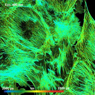
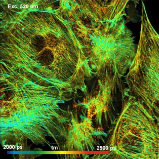
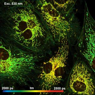
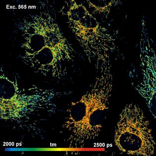
Fig. 29: Confocal FLIM with tuneable Intune laser. BPAE cells stained with Alexa 488 phalloidin and Mito Tracker Red. Amplitude weighted lifetime of double-exponential model. Excitation at 490, 520, 535, and 556 nm, all images 1024 x 1024 pixels.
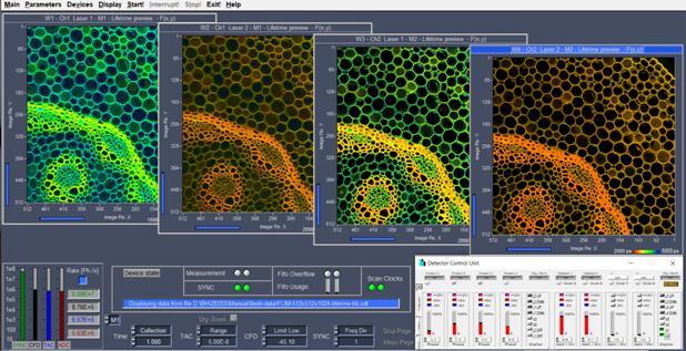
Fig. 30: FLIM at four combinations of excitation and emission wavelength. LSM 980 FLIM system with Laser Hub.
High Image Contrast up to the Highest Count Rates
Images taken with conventional TCSPC FLIM at high count rate often suffer from low intensity contrast. The reason is not the pile-up effect, as commonly believed, but intensity nonlinearity by the dead time of the TCSPC process. bh FLIM systems using the SPC-180 or SPC-QC-104 modules do not show this effect. The SPC-180 takes the intensity information from a fast parallel counter with almost no dead time, the SPC-QC-104 avoids dead time by a fast time-conversion method. An image taken at an average count rate of 6 MHz with an SPC-180NX is shown in Fig. 31. The peak count rate is about 10 MHz. The image on the left was recorded in the traditional TCSPC FLIM mode. Although it shows correct lifetimes it has lost almost all its intensity contrast. The image on the right was recorded in the 'Lifetime - Intensity' mode. It shows perfect intensity contrast.
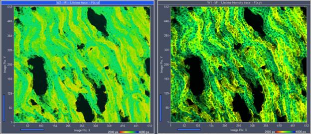
Fig. 31: Images of a mouse kidney sample taken at an average count rate of 6 MHz. Peak count rate is about 10 MHz. SPC-180 NX TCSPC / FLIM module. Left: Traditional TCSPC FLIM image. Right: Lifetime / Intensity mode, intensity from parallel counter channel.
Photon-Counting Intensity Images
A frequently asked question is whether a bh FLIM system can record conventional intensity images. Of course it can - the number of photons, and thus the intensity is part of the FLIM information contained in every pixel of a lifetime image. Recent FLIM systems using SPC-180 or SPC-QC-104 TCSPC modules even deliver the intensity without dead-time-induced nonlinearity. Intensity images can be displayed side by side with lifetime images, see Fig. 32.
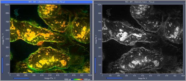
Fig. 32: Lifetime image (left) and intensity image (right), simultaneously displayed by SPCM. SPC-180N, lifetime-intensity mode.
Time-Series FLIM
Time-series FLIM is available for all system versions, and all detectors. The FLIM system performs a series of recordings and saves the results into consecutive data files. The principle is often called 'Record-and-Save' procedure. The advantage of the record-and-save procedure is it can be used for images of large numbers of pixels and time channels, and that the length of the series is virtually unlimited. The disadvantage is that some time has to be provided for data readout and data saving. This limits the speed of the sequence. In practice, the maximum reasonable speed is about 2 images per second [69]. For faster time series please see 'Express FLIM', page 26, and 'Temporal Mosaic FLIM', page 31. An example for time-series FLIM by the record-and save procedure is shown in Fig. 33.
Fig. 33: Time-series FLIM, recorded into sequence of files. Acquisition time 2 seconds per image. Chloroplasts in moss leaf, the lifetime changes due to the Kautski effect
Fast Acquisition
The Zeiss LSMs use fast beam scanning by galvanometer mirrors. A complete frame is scanned within a period of time from 50 ms to a few seconds. With a scan speed as fast as this the bh FLIM systems achieve surprisingly short acquisition times. An autofluorescence FLIM image of a live Enchytraeus albidus is shown in Fig. 34. The acquisition time was 1.2 seconds. Considering the high number of pixels, this is faster than what is achieved by many 'Fast FLIM' techniques [31, 75].
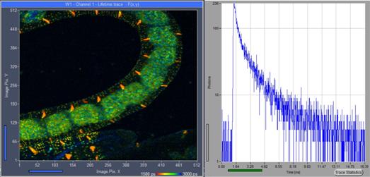
Fig. 34: Lifetime image taken from a live Enchytraeus albidus. Autofluorescence, 1.2 seconds acquisition time at 2 MHz average count rate and 50 MHz laser repetition rate. SPC‑QC‑104, 512 x 512 pixels. Online-FLIM with SPCM software. Decay curve in selected 10x10-pixel area shown on the right.
Express FLIM
Recording a typical TCSPC image within a short period of time requires an enormous data transfer rate from the TCSPC module to the computer. The data transfer problem increases if a longer sequence of images is to be recorded, and if several TCSPC channels are operated at high count rate simultaneously. bh have solved the problem by a technique called 'Express FLIM'. Express FLIM does not transfer data into the computer photon by photon. Instead, the hardware of the TCSPC module combines the information of all photons within a given pixel into a just two numbers. One is the first moment of the decay curve, the other the number of photons within the pixel. Both numbers are transferred to the computer at the end of each pixel. Even for fast scanning, the required data transfer rate can easily be achieved. The result is a lifetime image that contains first-moment values in the individual pixels. Express FLIM is available for all bh FLIM systems containing the SPC-QC-104 module. An example is shown in Fig. 35.
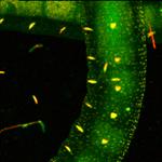
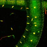
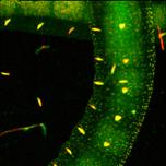
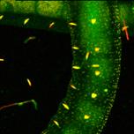
Fig. 35: Express-FLIM of a live Enchytraeus albidus. Autofluorescence, four subsequent images from a 5-frames/second sequence. SPC-QC-104, excitation pulse rate 80 MHz, average photon rate about 10×106 s-1.
FCS
The bh GaAsP hybrid detectors deliver highly efficient FCS [2, 27, 31]. Because the detectors are free of afterpulsing diffusion times are obtained from a single detector, without the loss in correlation events that occurs when the signals from two detectors are cross-correlated. FCS can be obtained with the diode-laser systems, the Intune system, and even with the multiphoton NDD systems. The bh SPCM data acquisition software calculates FCS online and fits the data with a user-configurable model function [31]. FCS can be recorded with picosecond lasers or with CW lasers. With ps excitation, the FCS procedure also delivers the decay function in the excited spot. The FCS recording can then be time-gated to prevent Raman signals from contaminating the FCS data. An example is shown in Fig. 36. Please see [36] or [2] for details.
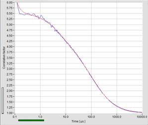
Fig. 36: FCS with HPM-100-40 hybrid detector. Decay curve and FCS curve. The first part of the decay has been suppressed by time-gating.
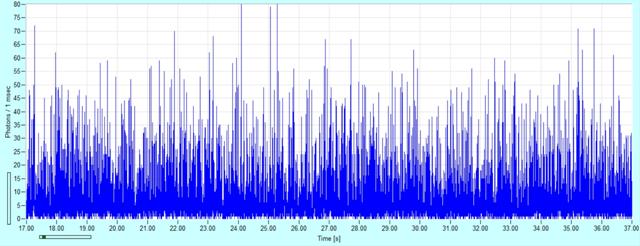
Fig. 37: Intensity trace recorded in parallel with FCS.
Detection of Nanoparticles
The parameter-tag mode of the FLIM system can also be used for single-particle detection. An example for the diffusion of fluorescent nanoparticles through the laser focus in shown in Fig. 38.
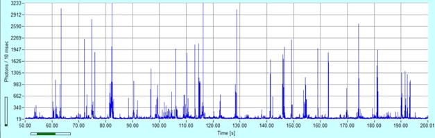
Fig. 38: Fluorescent nanoparticles drifting through the laser focus. Intensity trace.
The individual photon bursts can be further analysed by bh 'SPCDynamics' software, see Fig. 39. SPCDynamics displays fluorescence decay curves integrated over the bursts in a selected time interval, a phasor plot of the decay data of the bursts within a selected time interval, and decay curves and fluorescence lifetimes of individually selected bursts.
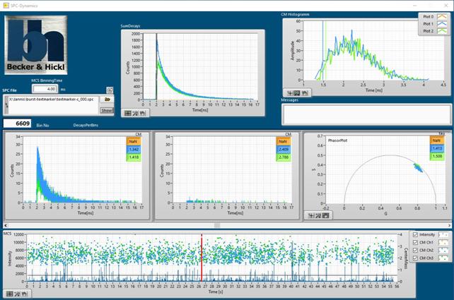
Fig. 39: Analysing photon bursts from single particles or single molecules by bh 'SPCDynamics' software
Precision Recording of Single Decay Curves
The DCS-120 system can record single decay curves from fluorophore solutions or from selected spots in a two-dimensional sample. Curves are obtained either in the 'Single' mode of SPCM, or from summing up the decay data from a multi-pixel area within a FLIM image. This makes a separate lifetime spectrometer for fluorophore characterisation unnecessary. Moreover: A multiphoton system with ultra-fast detectors beats any lifetime spectrometer in time resolution. An example is shown in Fig. 40.
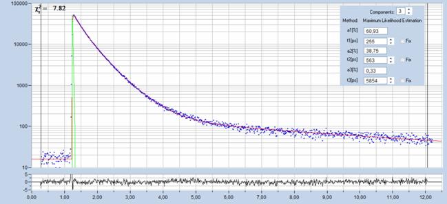
Fig. 40: Fluorescence decay curve recorded with a LSM 880 NLO. SPC-180N FLIM system with HPM-100-06 detector. Analysis by SPCImage NG.
Advanced FLIM Functions
Mosaic FLIM
Originally, bh introduced Mosaic FLIM to record large images with the Tile Imaging function of the Zeiss laser scanning microscopes [2, 31]. The microscope scans the sample by the TCSPC process illustrated in Fig. 8, page 9. In addition to fast beam scanning, it performs a raster stepping (Tile stepping) of consecutive areas of the sample by the sample stage. For every step the sample is scanned for a defined number of frames. For every step of the tile imaging, the TCSPC device records the data by its normal FLIM procedure. The memory is configured to provide space not only for a single image of the defined frame format but for the entire mosaic of tiles. The TCSPC FLIM process starts in the first tile, or mosaic element. After a defined number of frames the recording proceeds to the next mosaic element. Provided the number of frames per tile of the microscope stepping and the number of frames per mosaic elements are the same the TCSPC module records the entire mosaic into a single photon distribution. The recorded photon distribution represents a FLIM image of the entire mosaic. An example is shown in Fig. 41.
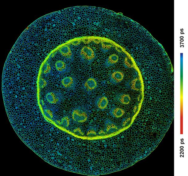
Fig. 41: Mosaic FLIM of a convallaria sample
The advantage of Mosaic FLIM is that a large sample area can be imaged with a microscope lens of high NA (numerical aperture). High NA delivers high spatial resolution and high detection efficiency, mosaic recording delivers a large field of view, a combination that cannot be obtained by beam scanning alone.
Temporal Mosaic FLIM
The idea that Mosaic FLIM records several images into one photon distribution leads to a more general concept of Mosaic FLIM: The transition from one mosaic element in the FLIM data to the next can be associated also to a change in another parameter of the experiment. An example is temporal mosaic FLIM. The sample is repeatedly scanned around the same spatial position, but subsequent images are recorded in consecutive elements of the FLIM mosaic. The result is a time series, the time step of which is a multiple of the frame time [31]. An example is shown in Fig. 42.
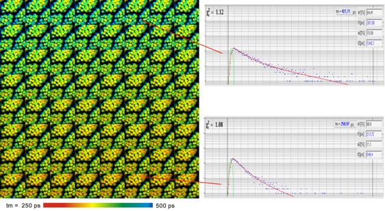
Fig. 42: Time series acquired by mosaic FLIM. Recorded at a speed of 1 mosaic element per second. 64 elements, each element 128 x 128 pixels, 256 time channels, double-exponential fit of decay data. Sequence starts at upper left. Moss leaf, lifetime changes by non-photochemical chlorophyll transient.
Temporal Mosaic FLIM with Triggered Accumulation
Compared to conventional time-laps FLIM temporal mosaic FLIM has several advantages: No time has to be reserved for the save operations, and the data can be better analysed with global-parameter fitting. The biggest advantage is, however, that mosaic time series data can be accumulated: A sample would be stimulated repeatedly by an external event, and the start of the mosaic recording be triggered with the stimulation. With every new stimulation the recording procedure runs through all elements of the mosaic, and accumulates the photons. Accumulation allows data to be recorded without the need of trading photon number and lifetime accuracy against the speed of the time series. Consequently, the time per step (or mosaic element) is only limited by the minimum frame time of the scanner. With the Zeiss LSMs, frame times (and thus time-series speeds) in the sub-50 ms range can be obtained. The technique is not only faster than any 'Fast FLIM' technique, it also avoids the need of excessively high excitation power and high count rate. Temporal Mosaic FLIM is thus an excellent way to investigate fast physiological processes in live systems [62, 61]. An example for recording Ca2+ transients in live neurons is shown in Fig. 43. Please see [31] for more information.
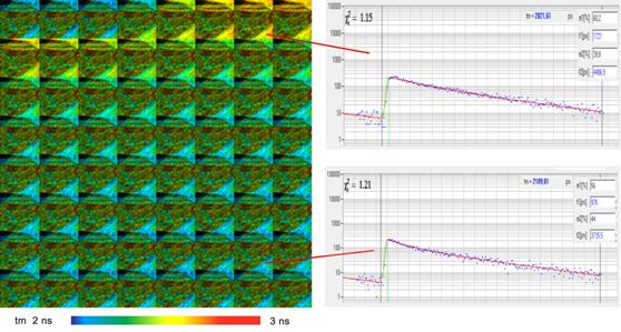
Fig. 43: Ca2+ transient in cultured neurons, incubated with Oregon Green Bapta. Electrical stimulation, stimulation period 3s, data accumulated over 100 stimulation periods. Time per mosaic element is 38 ms.
FLITS: Fluorescence Lifetime-Transient Scanning
Triggered Temporal Mosaic FLIM records image series at a speed of to 40 to 100 ms per image, or 10 to 25 images per second. Dynamic effects faster than that can be recorded by bh's FLITS procedure. FLITS records transient effects in the fluorescence lifetime of a sample along a one-dimensional scan. The maximum resolution at which lifetime changes can be recorded is given by the line scan time. With repetitive stimulation and triggered accumulation transient lifetime effects can be resolved at a resolution of about one millisecond [31, 28]. Typical applications are recording of chlorophyll transients and Ca2+ transients in neurons or neuronal tissue [30]. Examples are shown in Fig. 44 and Fig. 45.
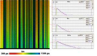
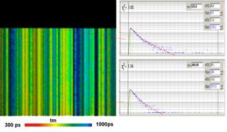
Fig. 44: FLITS of chloroplasts in a grass blade, change of fluorescence lifetime after start of illumination. Experiment time runs bottom up. Left: Non-photochemical transient, transient resolution 60 ms. Right: Photochemical transient. Triggered accumulation, transient-time resolution 1 ms.
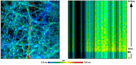
Fig. 45: FLITS of Ca2+ concentration in cultured neurons. Ca2+ sensor Oregon Green, LSM 7 MP, electrical stimulation, 100 stimulation periods accumulated. Transient-time resolution 2 ms.
Z Stack recording
Z stack recording with the bh FLIM systems for Zeiss LSM microscopes is achieved by controlling the Z drive of the microscope via the Zeiss ZEN software. Synchronisation with the Z scanning is obtained by a trigger pulse from the Zeiss system to the TCSPC / FLIM modules. The FLIM system has two procedures to record Z stacks. One is based on Mosaic FLIM: The data of subsequent planes are recorded in a large FLIM Mosaic. An example of a Mosaic-FLIM Z stack is shown in Fig. 46.
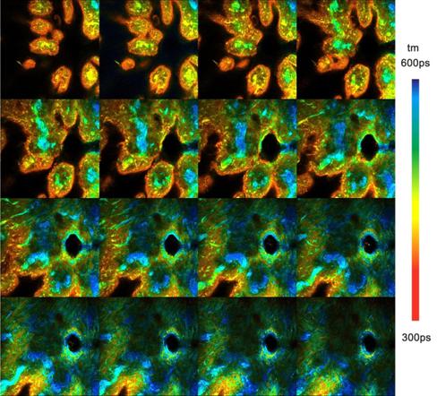
Fig. 46: Z stack of a pig skin sample, recorded by mosaic FLIM procedure.
The advantage of Mosaic Z stack recording is that the images of all Z planes are recorded in a single, large FLIM data set. This avoids delay by writing data in subsequent data sets, and guarantees that the data of all planes are exactly comparable. It also simplifies data analysis: The image segmentation functions of SPCImage can be applied to the entire Z stack, and all Z planes are analysed with exactly identical fit conditions. On the downside, the maximum number of planes is limited by the available data space. Depending on the desired lateral resolution, that means that 16 to 64 Z planes can be recorded.
A virtually unlimited number of Z planes can be recorded by a 'record and save' procedure. That means an image of the current plane is recorded, saved into a file, and then the focal plane is moved to the next Z plane. The procedure is repeated until the desired number of planes has been recorded. The advantage of the record-and-save procedure is that the frame size (pixels x time channels) can be made very large, and the number of Z planes is virtually unlimited. The disadvantage is that some time is required to save the data of the individual planes. An example of a high-resolution Z stack obtained from a fruit fly is shown below. The stack contains 126 planes, each scanned with 512 x 512 pixels and 1024 time channels. Fig. 47 shows a vertical projection of all planes in a single FLIM image by the 'Multi-File View' of SPCM.
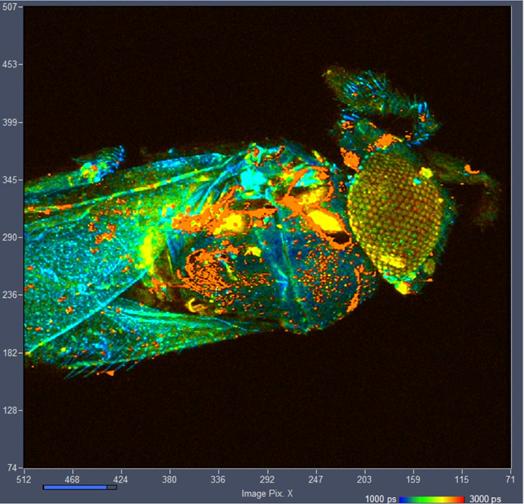
Fig. 47: Z Stack of a fruit fly. Vertical projection of all 126 planes of the z stack into a single FLIM image. Planes added by Multi-File View of SPCM, image displayed by Online-Lifetime function of SPCM. Single-exponential lifetime by first-moment analysis.
Fig. 48 shows the same data, analysed by SPCImage and combined into a 3D representation by Image J. All 126 planes were processed with a double-exponential model by the batch-processing function of SPCImage NG, and the resulting 126 tm images written into bmp files by the batch-export function. The bmp files were imported into Image J, which then constructed the 3D representation.
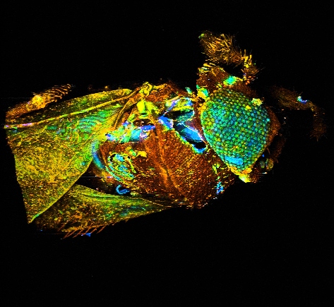
Fig. 48: Z stack of a fruit fly. Decay analysis by SPCImage NG and 3D reconstruction by ImageJ. Colour represents mean lifetime, tm, of double-exponential decay, lifetime range red to blue = 0 to 1250 ps.
Simultaneous FLIM / PLIM
The bh FLIM systems are able to simultaneously record fluorescence (FLIM) and phosphorescence lifetime images (PLIM) [13, 31, 66, 67, 71, 91]. The technique is based on modulating a high-frequency pulsed excitation laser synchronously with the pixel clock of the scanner. Photon times are determined both with reference to the laser pulses and the laser modulation period. Fluorescence is recorded during the on time, phosphorescence during the off time of the laser. The technique does not require a reduction of the laser repetition rate, works with two-photon excitation and non-descanned detection, and delivers an extremely high PLIM sensitivity. Unlike other PLIM techniques, it does not cause moiré in the images and can thus be used at scan rates no lower than the reciprocal phosphorescence decay time. For procedures and parameter setup in combination with the Zeiss LSMs please see [2]. A typical result is shown in Fig. 49. For application literature please see [31].
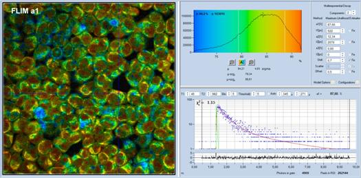
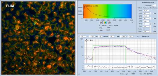
Fig. 49: Yeast cells stained with a Ruthenium dye. Top: NADH FLIM image and fluorescence decay curve in selected spot. Double-exponential analysis, metabolic indicator, a1, shown as pseudo colour. Bottom: Ruthenium PLIM image and phosphorescence decay curve in selected spot.
Excitation-Wavelength Multiplexing
It often happens that a sample contains two fluorophores which need to be excited at different wavelengths, either because the excitation spectra are too different, or because the emission cannot be cleanly separated if both are excited at the same wavelength [31]. A typical example is metabolic FLIM by recording signals from NAD(P)H and FAD [41, 43]. In principle, images of the two fluorophores could be recorded one after another. However, biological systems are dynamic, therefore it is desirable to record both images simultaneously. The bh FLIM systems use excitation-wavelength multiplexing for this task. The principle is shown in Fig. 50. Two lasers, Laser 1 and Laser 2, are multiplexed synchronously with the pixels, lines, or frames of the scan. The TCSPC modules receive information which of the lasers was active in the moment when a photon was detected. The modules then build up separate FLIM images for the two lasers. With two TCSPC modules and two detectors four images for different combinations of excitation and emission wavelength are obtained. In practice not all of these combinations may contain relevant data. Important is that the separation of the signals is near-ideal. Temporal overlap of the decay functions of the fluorophores as it occurs in pulse-by-pulse interleaved excitation does not exist.
Fig. 50: Excitation wavelength multiplexing. With two lasers and two TCSPC channels four images for different combinations of excitation and emission wavelength are obtained.
An example for the recording of a DAPI image simultaneously with an Alexa 488 image is shown in Fig. 11. Two laser wavelengths, 405 nm and 488 nm were multiplexed, and the data recorded in two parallel TCSPC channels, as shown in Fig. 50. The two FLIM images do no show any noticeable crosstalk in the signals of the two fluorophores.
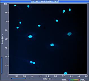
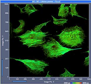
Fig. 51: BPAE sample with DAPI and Alexa 488, excited by multiplexed lasers at 405 nm (left) and 488 nm (right).
Multi-Wavelength FLIM
The principle shown in Fig. 8, page 9, can be extended to simultaneously detect in 16 wavelength channels. The optical spectrum of the fluorescence light is spread over an array of 16 detector channels. The TCSPC system determines the detection times, the channel numbers in the detector array, and the position, x, and y, of the laser spot for the individual photons. These pieces of information are used to build up a photon distribution over the time of the photons in the fluorescence decay, the wavelength, and the coordinates of the image [22, 24, 31, 26]. Applications are described in [52, 53, 54, 55, 83, 84], please see [31] for more references. The principle of multi-wavelength FLIM is shown in Fig. 52.

Fig. 52: Principle of Multi-Wavelength TCSPC FLIM
As for single-wavelength FLIM, the result of the recording process is an array of pixels. However, the pixels now contain several decay curves for different wavelength. Each decay curve contains a large number of time channels; the time channels contain photon numbers for consecutive times after the excitation pulse. An example is shown in Fig. 53.
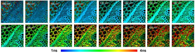
Fig. 53: Multi-wavelength FLIM of a convallaria sample
Multiphoton Multispectral NDD FLIM
The bh multi-wavelength detector is compatible with multiphoton excitation and non-descanned detection. It uses an optical interface that connects to the NDD ports of the LSM 710/780/880/980 NLO microscopes [26], see Fig. 7, page 8. A typical result is shown in Fig. 54.
Fig. 54: Multiphoton Multispectral NDD FLIM. Lifetime images and decay curves in selected pixels and wavelength channels. LSM 710 NLO, bh MW FLIM detector
Multispectral FLIM got a new push by the introduction of the new PML‑16 GaAsP 16-channel detector. This detector has five time the efficiency of the older PML‑16 detectors with conventional cathodes. Another improvement came from bhs Megapixel FLIM technology. Multi-spectral FLIM can now be obtained at an image size of 512 x 512 pixels in each wavelength channel while maintaining the usual 256-channel time resolution [31].
Near-Infrared FLIM: One-Photon Excitation by Ti:Sapphire Laser
Near-infrared (NIR) dyes are used as fluorescence markers in small-animal imaging and in diffuse optical tomography of the human brain. In these applications it is important to know whether the dyes bind to proteins or other tissue constituents, and whether their fluorescence lifetimes depend on the targets they bind to. There is also an increasing interest in FRET donors emitting in the near infrared and in near-infrared FRET-based molecular sensors for cell parameters. NIR FLIM is possible by using HPM‑100-50 detectors and Ti:Sapphire laser excitation. Different than for multiphoton FLIM, the Ti:Sapphire laser is used as a one-photon excitation source [11, 31, 37]. The Zeiss scan head does not contain a main dichroic beamsplitter for NIR excitation. However, it contains an 80/20 wideband beamsplitter. With the 80/20 beamsplitter FLIM images are obtained at reasonable efficiency, please see Fig. 55. The loss of 80% of the laser power at the beam splitter is insubstantial because the laser delivers far more power than needed.
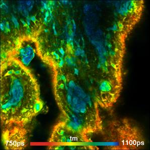
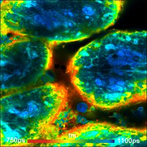
Fig. 55: Pig skin samples stained with 3,3-diethylthiatricarbocyanine. Excitation at 780nm, detection 800nm to 900nm
Near-Infrared FLIM: Multiphoton Excitation with OPO
With the Zeiss LSM NLO OPO systems near-infrared FLIM can be performed by two-photon excitation. The fluorescence signals are detected by HPM-100-50 NIR detectors and non-descanned detection. With two-photon excitation wavelengths in the range of 1000 to 1330 nm, the typical NIR dyes are excited at high efficiency [12, 31, 37]. Fluorescence is detected up to 900 nm. An example is shown in Fig. 56.
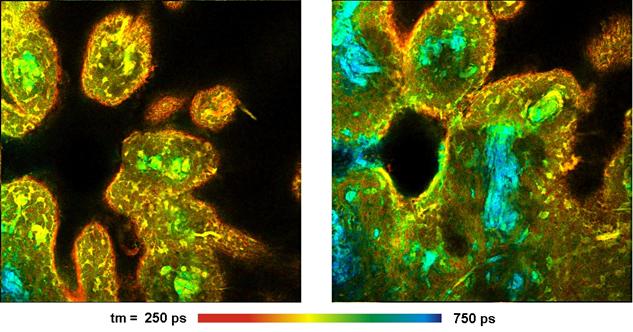
Fig. 56: Pig skin stained with Indocyanin Green. LSM 7 OPO system, two-photon excitation at 1200 nm, non-descanned detection, 780 to 850 nm. Depth from top of tissue 10 µm (left) and 40 µm (right). 512x512 pixels, 256 time channels.
FLIM Applications in Life Sciences
FLIM as a Molecular Imaging Technique
When fluorescence in a sample is excited the emission intensity depends, in first order, on the concentration of the fluorophore and the excitation power. Intensity imaging (Fig. 57, left) is thus an excellent way to resolve the spatial structure of a sample but it does not tell much about the interaction of the fluorophore with its molecular environment.
Spectral measurements or measurements in a few spectral channels (Fig. 57, middle) are able to distinguish between different fluorophores. However, they are not efficient in revealing changes in the molecular environment. Such changes usually do not cause large changes in the shape of the spectrum. Unless special fluorophores with several emission bands are used information on molecular effects is difficult to obtain.
The situation is different for the fluorescence lifetime. The fluorescence lifetime of a fluorophore (Fig. 57, right), does, of course depend on the type of the fluorophore. However, within reasonable limits, it does not depends on the concentration and the excitation power. Instead, it changes systematically and predictably with the molecular environment of the fluorophore. By using the fluorescence lifetime, or, more precisely, the shape of the fluorescence decay function, molecular effects can therefore be investigated independently of the unknown and, usually, variable fluorophore concentration.
Fig. 57: Fluorescence. Left to right: Excitation light is absorbed by a fluorophore, and fluorescence is emitted at a longer wavelength. The fluorescence intensity varies with concentration. The fluorescence spectrum is characteristic of the type of the fluorophore. The fluorescence decay function is an indicator of interaction of the fluorophore with its molecular environment.
Frequent FLIM applications are measurements of the molecular environment of the fluorophores, such as pH and concentration of biologically relevant ions, probing of protein interaction via FRET, and investigation of the metabolic state of cell and tissues via the fluorescence lifetimes of NADH and FAD. FLIM may also find application in plant physiology because the fluorescence lifetime of chlorophyll changes with the photosynthesis activity.
Molecular Parameters - Derived from Fluorescence-Decay Data
Molecular environment parameters, such as local pH [65], ion concentrations [63, 68], local viscosity [70, 73] or redox potential are available through TCSPC FLIM and precision decay analysis [6, 32]. With appropriate calibration of the probe the results are quantitative, i.e. independent of the laser power, the fluorophore concentration, the parameters of the optical-system, and other instrumental details. Examples are shown in the figures below. Please see [72, 95] for more applications.
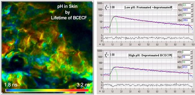
Fig. 58: Lifetime image of skin tissue stained with BCECF. The lifetime is an indicator of the pH. Right: Fluorescence decay curves in an area of low pH (top) and high pH (bottom). LSM 510 NLO, Data Courtesy of Theodora Mauro, University of San Francisco.
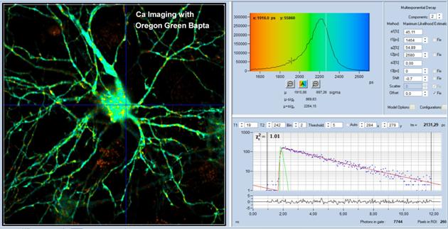
Fig. 59: FLIM image of cultured neuron stained with Oregon green OGB-1 AM. Colour range from tm = 1200 ps (blue) to 2400 ps (red). Decay curves of regions with low Ca (top) and high Ca (bottom) shown on the right. LSM 7 MP, Data courtesy of Inna Slutsky and Samuel Frere, Tel Aviv University, Sackler School of Medicine.
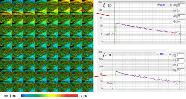
Fig. 60: Ca2+ transient in cultured neurons. Oregon Green Bapta, data recorded by temporal mosaic FLIM, Mosaic FLIM with triggered accumulation, 38 ms per mosaic element. Zeiss LSM 7 MP, bh Simple-Tau 152 TCSPC FLIM system. Data courtesy of Inna Slutsky and Samuel Frere, Tel Aviv University, Sackler School of Medicine.
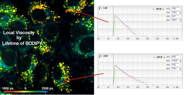
Fig. 61: Local viscosity, detected by lifetime of BODIPY-based sensor
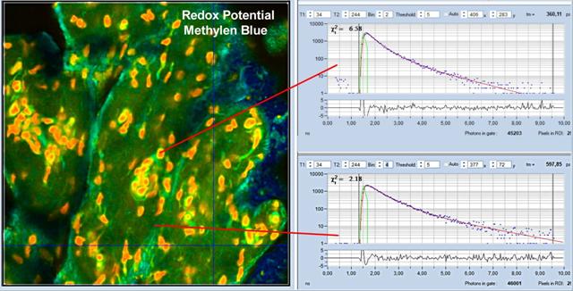
Fig. 62: Redox potential, detected by lifetime of Methylen Blue
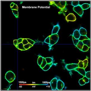
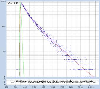
Fig. 63: Measurement of Membrane-Potential [31, 35]. FLIM image of HEK cells loaded with a voltage-sensitive dye, decay curve in selected 12x12 pixel area. LSM 980 with bh FLIM system and bh Laser Hub. Data courtesy of Susanna Yaeger-Weiss, University of Berkeley
FRET - Results from a Single Donor FLIM Image
FRET (Förster Resonance Energy Transfer) [59, 60] is used to probe protein interaction and protein structure in biological systems. The excitation energy is absorbed by a donor. It then transfers to an acceptor, and is emitted via the emission band of the acceptor. The energy transfer occurs only if the distance between the donor and the acceptor is less than a few nm. FRET is used to obtain information about protein interaction, protein folding, and protein structure. In principle, FRET measurements can be performed by comparing donor intensities with and without an acceptor [79]. However, intensity-FRET measurements are difficult to calibrate. FRET measurements are therefore mainly performed by FLIM [23, 31, 51, 58, 80, 82]. When FRET occurs the donor is losing energy to the acceptor, and its fluorescence lifetime becomes shorter than for the donor alone. The decrease in the donor lifetime is then a measure for the FRET intensity. FLIM FRET is usually considered to be inherently quantitative. In fact, it is not, especially when it is based on simple single-exponential 'fluorescence lifetimes' [33].
Quantitative FLIM FRET results are obtained in combination with double-exponential FRET analysis. The method has been developed by bh already in 2005 and has been constantly improved in the past years. The principle is shown in Fig. 64. It is based on the fact that the fluorescence decay function of the donor contains a component from interacting donor and from non-interacting donor. The amplitudes and the lifetimes of the components are determined by double-exponential decay analysis. The parameters are then used to calculate the classic FRET efficiency, the FRET efficiency of the interacting donor, the amount of interacting donor, and the donor-acceptor distance. Please see [32, 34] for details.
Fig. 64: Fluorescence decay components in FRET systems
In contrast to single-exponential FRET techniques, the method delivers correct FRET efficiencies and FRET distances even for incomplete donor-acceptor linking, and, importantly, without the need of reference data from a donor-only sample [31, 34].
The classic (average) FRET efficiency, the FRET efficiency of the interacting donor, the amount of interacting donor, and the donor-acceptor distance are displayed directly by SPCImage NG [32]. An example is shown in Fig. 65. For details and for a review of the FLIM FRET literature please see [31].
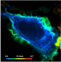
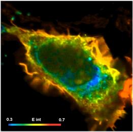
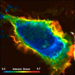
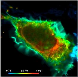
Fig. 65: FRET Measurement in life cell. Classic FRET efficiency, FRET efficiency of interacting donor, amount of interacting donor, and ratio of donor-acceptor distance to Förster radius. bh double-exponential FRET technique, LSM-880 with bh picosecond diode laser and SPC-152 FLIM system, SPCImage NG data analysis.
Metabolic Imaging by NADH FLIM
For several decades, it has been attempted to obtain metabolic information from the fluorescence lifetime of NADH (nicotinamide adenine dinucleotide). These attempts were not successful in deriving the metabolic state because the lifetimes of the NADH decay components depend also on molecular parameters other than the metabolic state. bh FLIM systems have overcome the problem by using the ratio of bound/unbound NADH [78, 93] or bound/unbound FAD. Because the bound and unbound forms have different fluorescence lifetimes this ratio is represented by the amplitude ratio of the decay components (a1/a2) or the amplitude of the fast decay component, a1. It turns out that a1/a2 (the metabolic ratio) or a1 (the metabolic indicator) describe the metabolic state independently of the type of the cell and its molecular environment. In most cells and tissues, tumor cells have an a1 above 0.7, whereas normal cells have an a1 below 0.7 [43, 94]. An example is shown in Fig. 66. For references on applications please see [31].
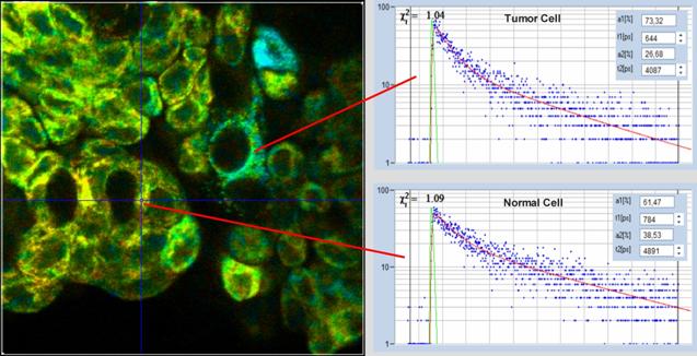
Fig. 66: Metabolic FLIM, a1 image and decay curves. Live human bladder cells from a biopsy. Upper curve: Tumor cell. Lower curve: Normal cell. The tumor cell has an a1 above 0.7. Zeiss Axio Observer with bh DC-120 scan head. Data analysis with SPCImage NG, MLE algorithm.
NADH FLIM for Clinical Diagnostics
It has been shown that NADH FLIM can be used for clinical diagnostics. FLIM data were obtained from human bladder cells excised during surgery. The patients had been diagnosed with bladder cancer or other suspicious lesions by classic endoscopy. Measurements on the excised material were performed immediately after surgery, before the material went to histology [94]. By using a normal / cancer discrimination threshold of a1 = 0.71 perfect agreement with the histology results was obtained. Please see [31, 43, 94] for details.
Personalised Chemotherapy
NADH FLIM is closely related to effect of cancer drugs in chemotherapy [92]. Skala and Walsh used Metabolic FLIM to evaluate the effect of different cancer drugs on cells from biopsies from patients, and to develop the best treatment strategy [96, 97]. The cells are cultured, the cell cultures are treated with the drugs, the cells are repeatedly imaged by metabolic FLIM. Within a few days, the most efficient drug can be determined and a treatment strategy for the patient be developed. If the technique can be transferred into clinical use - which is technically easily possible - it has the potential to revolutionise cancer treatment.
Metabolic Imaging of Skin
Metabolic FLIM can be applied to the investigation of tumor progression in mammalian skin [56, 77, 85, 86, 87]. Fig. 67 and Fig. 68 show NADH images of mouse skin. Fig. 67 shows healthy skin, Fig. 68 skin from the boarder of a tumor. Both images show the amplitude of the fast decay component, a1. It can be seen clearly that a1 is shifted to higher values in the tissue from the vicinity of the tumor, see histogram of a1 in the upper right of the panels.
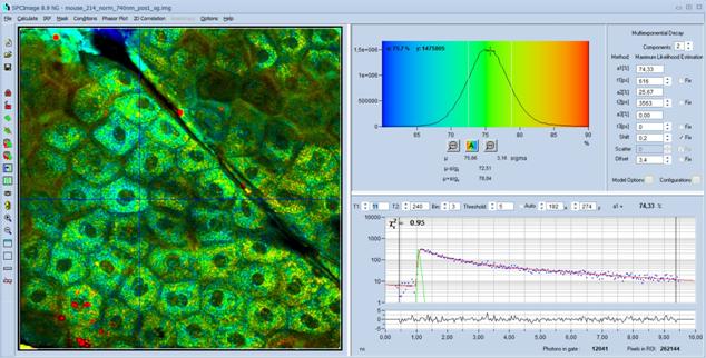
Fig. 67: Mouse skin, NADH image, double-exponential decay analysis, colour-coded image of the amplitude, a1, of the fast decay component. SPC-150 FLIM system, LSM 880 NLO, two-photon excitation at 750 nm. Data analysis with SPCImage NG.
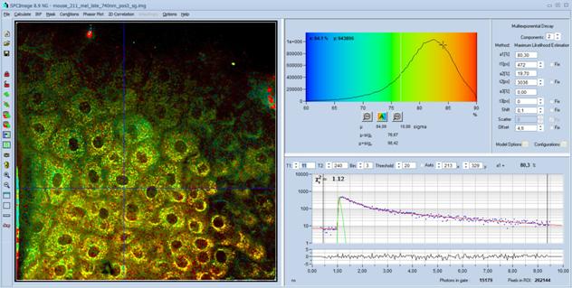
Fig. 68: Mouse skin, NADH image, double-exponential decay analysis, colour-coded image of the amplitude, a1, of the fast decay component. SPC-150 FLIM system, LSM 880 NLO, two-photon excitation at 750 nm. Data analysis with SPCImage NG.
Malignant Melanoma
Malignant melanoma manifest in FLIM data by a decay component of extremely short fluorescence lifetime and high amplitude [48]. Fig. 69 shows a lifetime image of a vertical section through malignant-melanoma tissue. Superficial layers are shown on the right in the image, deeper layers on the left. Colour coding shows the lifetime of the fast decay component, t1, obtained by fitting the decay data by a triple-exponential model. Decay curves from selected spots of the image are shown on the right. The sharp peak in the decay curve from the superficial layer (bottom, right) shows visibly that there must be an extremely fast decay component. The fit delivers a lifetime, t1, of 13 ps and an amplitude, a1, of 98% for this component. The amplitude ratio, a1/(a2+a3), is about 57, which is unusually high for biological material. The peak is not present in the decay curve from deep tissue layers, see top right. The component lifetimes in these areas are in a more or less 'normal' range, and compatible with a mixture of NADH, FAD, and, possibly, FMN [42]. The parameters are t1 = 185 ps, a1 = 23.8%, a1/(a2+a3) = 0.31.
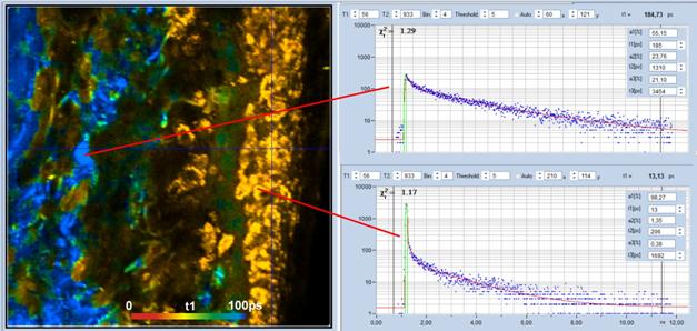
Fig. 69: Vertical section through melanoma tissue. Colour-coded image of the lifetime of the fast component, t1, of a triple-exponential fit of the data. Red to blue corresponds to 0 to 100 ps. Decay curves in characteristic spots of the image are shown on the right. LSM 880 NLO with SPC-150NX FLIM system, Data analysis by SPCImage NG.
For comparison, Fig. 70 shows a FLIM image of a sample from a benign pigmented lesion. A tm image is shown on the left, a decay curve from a selected spot on the right. As can be seen from the figure there is no ultra-fast component of high amplitude, as in the melanoma data. The fast decay component has a lifetime of 96 ps, and an amplitude of 45%. This is fast, but not as fast as in the malignant melanoma. The amplitude ratio, a1/(a2+a3), is about 0.8, i.e. 70 times smaller than for the malignant melanoma.
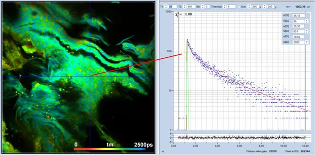
Fig. 70: Left: tm image of a sample from a benign pigments skin lesion. Red to blue corresponds to tm = 0 ps to 2500 ps. Right: decay curve in a selected spot of the image. There is no high-amplitude ultra-fast decay component.
Nanoparticles in Skin
An important issue in dermatology is diffusion of drugs and nano-particles through human skin. On the one hand, diffusion through the skin may be desirable as a pathway of drug delivery. On the other hand, nanoparticles contained in sunscreens or cosmetic products should not permeate through the stratum corneum of human skin. Moreover, it is important whether the nanoparticles cause changes in their molecular environment. The use of FLIM to study these effects has been described in [74, 81, 87]. For additional references please see [31].
Autofluorescence of the Ocular Fundus
TCSPC FLIM has recently been introduced in ophthalmic scanners [31]. The instruments have produced FLIM images of amazing quality. Clinical trials have shown that FLIM is able to detect metabolic changes that are early indications of a number of eye diseases [64, 76, 88, 90]. Ophthalmic scanners do, however, not deliver spatial resolution at the cell level. Clinical research has therefore to be supported by FLIM microscopy of ex-vivo samples.
A FLIM microscopy study of extra-macular drusen has been published by Schweitzer et al. [89]. Based on the FLIM data, the authors were able to discriminate the RPE from Bruchs membrane, drusen, and choroidal connective tissue. An example of a FLIM image of the RPE with hard drusen is shown in Fig. 71. The data were acquired with the MW FLIM multi-wavelength detector. Fig. 71 shows the lifetime data in all combined wavelength channels. Triple-exponential decay analysis was used; the images show the fast decay component, the medium component, and the slow decay component. Interestingly, in the drusen and in the Bruchs membrane an extremely slow component with about 8 ns decay time occurs. The lifetimes in the RPE are much shorter.
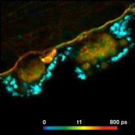
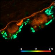
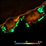
Fig. 71: Autofluorescence FLIM image of a human fundus sample. Triple-exponential analysis, left to right: Lifetimes of the fast, medium, and slow decay component. Courtesy of Dietrich Schweitzer, Martin Hammer, Sven Peters, Christoph Biskup, University Jena, Germany. LSM 710, bh MW FLIM detector and SPC‑150 TCSPC module.
Spectrally resolved data are shown in Fig. 72. It shows 6 consecutive wavelength channels of the MW FLIM detector from 450 nm to 575 nm. The lifetime shown is the amplitude weighted average of a triple-exponential decay model. The intensities were normalised to the brightest pixel.
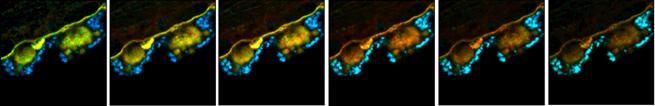
Fig. 72: Lifetime images of the amplitude-weighted lifetime, tm, for single wavelength channels from 450 nm to 575 nm. The lifetime scale is blue to red, 0 to 2500 ps. LSM 710, bh MW FLIM detector and SPC‑150 TCSPC module.
Summary
The bh FLIM systems for Zeiss LSM 710/780/880/980 laser scanning microscopes are high-performance lifetime imaging system based on laser scanning and multi-dimensional TCSPC. The systems are characterised by high time resolution, high sensitivity, high photon efficiency, fast acquisition, high spatial resolution, and suppression of out-of-focus fluorescence and laterally and longitudinally scattered light. bh FLIM systems can be used for the entire range from entry level FLIM to high-end multidimensional molecular imaging applications.
Different than other FLIM techniques and FLIM systems which consider FLIM just a way to improve contrast in laser scanning microscopy, the bh FLIM systems have strictly been designed with molecular-imaging applications in mind. The systems thus have capabilities beyond the reach of other systems: Compatibility with live-cell imaging, extraordinarily high time resolution and photon efficiency, improved capability to split decay functions into several components, excitation-wavelength multiplexing in combination with parallel-channel detection, recording of dynamic lifetime changes, and simultaneous FLIM/PLIM. Typical applications are measurements of molecular-environment parameters, protein-interaction experiments by FRET techniques, label-free imaging, imaging of the metabolic state of cells and tissues, the use of endogenous fluorophores with lifetimes in the 10-ps range, oxygen-concentration measurement, and recording of fast physiological processes in biological systems. No other FLIM technique and no other FLIM system offers a similar range of capabilities.
References
1. S. R. Alam, H. Wallrabe, Z. Svindrych, A. K. Chaudhary, K. G. Christopher, D. Chandra, A. Periasamy, Investigation of Mitochondrial Metabolic Response to Doxorubicin in Prostate Cancer Cells: An NADH, FAD and Tryptophan FLIM Assay. Scientific Reports 7 (2017)
2. Becker & Hickl GmbH, Modular FLIM systems for Zeiss LSM 710/780/880 family laser scanning microscopes. User handbook, 8th ed., available on www.becker-hickl.com, please contact bh for printed copies
5. Becker & Hickl GmbH, LHB-104 Laser Hub. User manual, available on www.becker-hickl.com.
7. Becker & Hickl GmbH, Becker & Hickl GmbH, Megapixel FLIM with bh TCSPC Modules - The New SPCM 64-bit Software. Application note, available on www.becker-hickl.com
8. Becker & Hickl GmbH, FLIM with NIR Dyes. Application note, available on www.becker-hickl.com
11. Becker & Hickl GmbH, FLIM with NIR Dyes. Application note, available on www.becker-hickl.com
21. W. Becker, K. Benndorf, A. Bergmann, C. Biskup, K. König, U. Tirlapur, T. Zimmer, FRET measurements by TCSPC laser scanning microscopy, Proc. SPIE 4431, 94-98 (2001)
22. W. Becker, A. Bergmann, C. Biskup, T. Zimmer, N. Klöcker, K. Benndorf, Multi-wavelength TCSPC lifetime imaging, Proc. SPIE 4620 79-84 (2002)
23. W. Becker, A. Bergmann, M.A. Hink, K. König, K. Benndorf, C. Biskup, Fluorescence lifetime imaging by time-correlated single photon counting, Micr. Res. Techn. 63, 58-66 (2004)
24. W. Becker, Advanced time-correlated single-photon counting techniques. Springer, Berlin, Heidelberg, New York, 2005
25. W. Becker, A. Bergmann, E. Haustein, Z. Petrasek, P. Schwille, C. Biskup, L. Kelbauskas, K. Benndorf, N. Klöcker, T. Anhut, I. Riemann, K. König, Fluorescence lifetime images and correlation spectra obtained by multi-dimensional TCSPC, Micr. Res. Tech. 69, 186-195 (2006)
26. W. Becker, A. Bergmann, C. Biskup, Multi-Spectral Fluorescence Lifetime Imaging by TCSPC. Micr. Res. Tech. 70, 403-409 (2007)
30. W. Becker, V. Shcheslavskiy, S. Frere, I. Slutsky, Spatially resolved recording of transient fluorescence lifetime effects by line-scanning TCSPC. Microsc. Microsc. Res. Techn. 77, 216-224 (2014)
31. W. Becker, The bh TCSPC handbook. 10th edition. Becker & Hickl GmbH (2023). Available on www.becker-hickl.com, please contact bh for printed copies.
35. W. Becker, A. Bergmann, Measurement of Membrane Potentials in Cells by TCSPC FLIM. Application note (2023), available on www.becker-hickl.com
39. W. Becker, Introduction to Multi-Dimensional TCSPC. In W. Becker (ed.) Advanced time-correlated single photon counting applications. Springer, Berlin, Heidelberg, New York (2015)
40. W. Becker, V. Shcheslavskiy, H. Studier, TCSPC FLIM with Different Optical Scanning Techniques, in W. Becker (ed.) Advanced time-correlated single photon counting applications. Springer, Berlin, Heidelberg, New York (2015)
46. W. Becker, A. Bergmann, C. Junghans, Ultra-Fast Fluorescence Decay in Natural Carotenoids. Application note, www. becker-hickl.com (2022)
49. T. S. Blacker, Z. F. Mann, J. E. Gale, M. Ziegler, A. J. Bain, G. Szabadkai, M. R. Duchen, Separating NADH and NADPH fluorescence in live cells and tissues using FLIM. Nature Communications 5, 3936-1 to -6 (2014)
50. Carl Zeiss MicroImaging GmbH, Take the BiG Step Towards Universal Detection. www.zeiss.de/LSM
51. Y. Chen, A. Periasamy, Characterization of two-photon excitation fluorescence lifetime imaging microscopy for protein localization, Microsc. Res. Tech. 63, 72-80 (2004)
52. D. Chorvat, A. Chorvatova, Spectrally resolved time-correlated single photon counting: a novel approach for characterization of endogenous fluorescence in isolated cardiac myocytes. Eur. Biophys. J. 36:73-83 (2006)
58. R.R. Duncan, A. Bergmann, M.A. Cousin, D.K. Apps, M.J. Shipston, Multi-dimensional time-correlated single-photon counting (TCSPC) fluorescence lifetime imaging microscopy (FLIM) to detect FRET in cells, J. Microsc. 215, 1-12 (2004)
59. Th. Förster, Zwischenmolekulare Energiewanderung und Fluoreszenz, Ann. Phys. (Serie 6) 2, 55-75 (1948)
61. S. Frere, I. Slutsky, Calcium imaging using Transient Fluorescence-Lifetime Imaging by Line-Scanning TCSPC. In: W. Becker (ed.) Advanced time-correlated single photon counting applications. Springer, Berlin, Heidelberg, New York (2015)
63. Th. Gensch, V. Untiet, A. Franzen, P. Kovermann, C. Fahlke, Determination of Intracellular Chloride Concentrations by Fluorescence Lifetime Imaging. In: W. Becker (ed.) Advanced time-correlated single photon counting applications. Springer, Berlin, Heidelberg, New York (2015)
64. Dysli, C., Wolf, S., Berezin, M.Y., Sauer, L., Hammer, M., Zinkernagel, M.S., Fluorescence lifetime imaging ophthalmoscopy, Progress in Retinal and Eye Research (2017), doi: 10.1016/j.preteyeres.2017.06.005
65. K.M. Hanson, M.J. Behne, N.P. Barry, T.M. Mauro, E. Gratton, Two-photon fluorescence imaging of the skin stratum corneum pH gradient, Biophys. J. 83, 1682-1690 (2002)
66. J. Jenkins, R. I. Dmitriev, D. B. Papkovsky, Imaging Cell and Tissue O2 by TCSPC-PLIM. In: W. Becker (ed.) Advanced time-correlated single photon counting applications. Springer, Berlin, Heidelberg, New York (2015)
67. S. Kalinina, V. Shcheslavskiy, W. Becker, J. Breymayer, P. Schäfer, A. Rück, Correlative NAD(P)H-FLIM and oxygen sensing-PLIM for metabolic mapping. J. Biophotonics 9(8):800-811 (2016)
68. H. Kaneko, I. Putzier, S. Frings, U. B. Kaupp, and Th. Gensch, Chloride Accumulation in Mammalian Olfactory Sensory Neurons, J. Neurosci., 24(36) 7931-7938 (2004)
70. M. K. Kuimova, G. Yahioglu, J. A. Levitt, K. Suhling, Molecular Rotor Measures Viscosity of Live Cells via Fluorescence Lifetime Imaging. J. Am. Chem. Soc. 130, 66726673 (2008)
72. J.R. Lakowicz, Principles of Fluorescence Spectroscopy, 3rd edn., Springer (2006)
76. Y. Miura, G. Hüttmann, R. Orzekowsky-Schroeder, P. Steven, M. Szszak, N. Koop, R. Brinkmann, Two-photon microscopy and fluorescence lifetime imaging of retinal pigment epithel cells under oxydative stress. Invest Ophthalmol Vis Sci, IOVS 54, 3366-3377 (2013)
78. R.J. Paul, H. Schneckenburger, Oxygen concentration and the oxidation-reduction state of yeast: Determination of free/bound NADH and flavins by time-resolved spectroscopy, Naturwissenschaften 83, 32-35 (1996)
79. A. Periasamy, Methods in Cellular Imaging. Oxford University Press, Oxford New York (2001)
80. A. Periasamy, N. Mazumder, Y. Sun, K. G. Christopher, R. N. Day, FRET Microscopy: Basics, Issues and Advantages of FLIM-FRET Imaging. In: W. Becker (ed.) Advanced time-correlated single photon counting applications. Springer, Berlin, Heidelberg, New York (2015)
81. Tarl W. Prow, Jeffrey E. Grice, Lynlee L. Lin, Rokhaya Faye, Margaret Butler, Wolfgang Becker, Elisabeth M.T. Wurm, Corinne Yoong, Thomas A. Robertson, H. Peter Soyer, Michael S. Roberts, Nanoparticles and microparticles for skin drug delivery. Advanced Drug Delivery Reviews 63, 470491 (2011)
82. L. Richert, P. Didier, H. de Rocquigny, Y. Mély, Monitoring HIV-1 Protein Oligomerization by FLIM FRET Microscopy. In: W. Becker (ed.) Advanced time-correlated single photon counting applications. Springer, Berlin, Heidelberg, New York (2015)
83. A. Rück, Ch. Hülshoff, I. Kinzler, W. Becker, R. Steiner, SLIM: A New Method for Molecular Imaging. Micr. Res. Tech. 70, 403-409 (2007)
85. W.Y. Sanchez, T.W. Prow, W.H. Sanchez, J.E.Grice, M.S. Roberts, Analysis of the metaboloic deterioration of ex-vivo skin, from ischemic necrosis, through the imaging of intracellular NAD(P)H by multiphoton tomography and fluorescence lifetime imaging microscopy (MPT-FLIM). J. Biomed. Opt. 09567RR in press (2010)
87. W. Y. Sanchez, M. Pastore, I. Haridass, K. König, W. Becker, M. S. Roberts, Fluorescence Lifetime Imaging of the Skin. In: W. Becker (ed.) Advanced time-correlated single photon counting applications. Springer, Berlin, Heidelberg, New York (2015)
88. D. Schweitzer, S. Schenke, M. Hammer, F. Schweitzer, S. Jentsch, E. Birckner, W. Becker, Towards Metabolic Mapping of the Human Retina. Micr. Res. Tech. 70, 403-409 (2007)
95. K. Suhling, L. M. Hirvonen, J. A. Levitt, P.-H. Chung, C. Tregido, A. le Marois, D. Rusakov, K. Zheng, Fluorescence Lifetime Imaging (FLIM): Basic Concepts and Recent Applications. In: W. Becker (ed.) Advanced time-correlated single photon counting applications. Springer, Berlin, Heidelberg, New York (2015)
96. A. J. Walsh, R. S. Cook, M. E. Sanders, L. Aurisicchio, G. Ciliberto, C. L. Arteaga, M. C. Skala, Quantitative Optical Imaging of Primary Tumor Organoid Metabolism Predicts Drug Response in Breast Cancer. Cancer Res 74, OF1-OF11 (2014)
97. A. J. Walsh, A. T. Shah, J. T. Sharick, M. C. Skala, Fluorescence Lifetime measurements of NADH in live cells and tissue. In: W. Becker (ed.) Advanced time-correlated single photon counting applications. Springer, Berlin, Heidelberg, New York (2015)
Specifications
General Principle
Lifetime measurement time-domain
Excitation high-frequency pulsed lasers
Buildup of lifetime images Single-photon detection by multi-dimensional TCSPC [31]
Builds up distribution of photons over photon arrival time
after laser pulses, scan coordinates,
time from laser modulation, time from start of experiment.
Multi-wavelength FLIM uses wavelength of photons as additional coordinate of photon distribution
Excitation wavelength multiplexing uses laser number as additional coordinate of photon distribution
Scan rate works at any scan rate
Buildup of fluorescence correlation data correlation of absolute photon times [31]
General operation modes FLIM, two spectral or polarisation channels
Multi-wavelength FLIM
Time-series FLIM, microscope-controlled time series
Z-Stack FLIM
Mosaic FLIM, x,y, z, temporal
Excitation-wavelength multiplexed FLIM
FLITS (fluorescence lifetime-transient scanning)
PLIM (phosphorescence lifetime imaging) simultaneous with FLIM
FCS, cross FCS, gated FCS, PCH
Single-point fluorescence decay recording
Data recording hardware, please see [31] for details
TCSPC System SPC-150NX or SPC-180NX TCSPC / FLIM modules
Number of parallel TCSPC / FLIM channels typ. 2, min. 1, max 4
Number of detector (routing) channels in FLIM modes 16 for each FLIM channel
Principle Advanced TAC/ADC principle
Electrical time resolution 1.63 ps rms / 3.5 ps fwhm
Minimum time channel width 405 fs
Timing stability over 30 minutes typ. better than 5ps
Dead time SPC-150NX: 100 ns / SPC-180NX: 80 ns
Saturated count rate 10 MHZ / 12 MHz per channel
Dual-time-base operation via micro times from TAC and via macro time clock
Source of macro time clock internal 40MHz clock or from laser
Input from detector constant-fraction discriminator
Reference (SYNC) input constant-fraction discriminator
Synchronisation with scanning via frame clock, line clock and pixel clock pulses
Scan rate any scan rate
Synchronisation with laser multiplexing via routing function
Recording of multi-wavelength data simultaneous in 16 channels, via routing function
Experiment trigger function TTL, used for Z stack FLIM and microscope-controlled time series
Basic acquisition principles on-board-buildup of photon distributions
buildup of photon distributions in computer memory
generation of parameter-tagged single-photon data
online auto or cross correlation and PCH
Operation modes f(t), oscilloscope, f(txy), f(t,T), f(t) continuous flow
FIFO (correlation / FCS / MCS) mode
Scan Sync In imaging, Scan Sync In with continuous flow
FIFO imaging, with MCS imaging, mosaic imaging, time-series imaging
Multi-detector operation, laser multiplexing operation
cycle and repeat function, autosave function
Max. Image size, pixels (SPCM 64 bit software) 4096x4096 2048x2048 512x512 256x256
No of time channels, see [31] 64 256 1024 4096
Data Acquisition Software, please see [31] for details
Operating system Windows 10, 64 bit
Loading of system configuration single click in predefined setup panel
Start / stop of measurement by operator or by timer, starts with start of scan, stops with end of frame
Online calculation and display, FLIM, PLIM in intervals of Display Time, min. 1 second
Online calculation and display, FCS, PCH in intervals of Display Time, min. 1 second
Number of images displayed simultaneously max 8
Number of curves (Decay, FCS, PCH, Multiscaler) 8 in one curve window
Cycle, repeat, autosave functions user-defined, used for
for time-series recording, Z stack FLIM,
microscope-controlled time series
Saving of measurement data User command or autosave function
Optional saving of parameter-tagged single-photon data
Link to SPCImage data analysis automatically after end of measurement or by user command
Data Analysis: bh SPCImage, integrated in bh TCSPC package, see [2] or [31]
Data types processed FLIM, Lif/Int FLIM, PLIM, MW FLIM, Mosaic FLIM, time-series, Z stacks, single curves
Procedures WLS, MLE or first-moment calculation
GPU Processing MLE, if GPU is present
Extra Hardware NVIDIA GPU, optional
IRF Synthetic IRF or measured IRF
Model functions Single, double, triple exponential decay
Single, double, triple exponential incomplete decay models
Shifted-component model
Parameters displayed Amplitude- or intensity-weighted average of component lifetimes
Component lifetimes, component amplitudes, ratios of lifetimes or amplitudes
Classic and interacting-donor FRET efficiency, donor-acceptor distance
Fractional intensities of components or ratios of fractional intensities
Parameter distributions
Phasor Plot Available for all types of FLIM data
Parameter histograms, one-dimensional Pixel frequency over any decay parameter or ratio of decay parameters
Parameter histograms, two-dimensional Pixel frequency over two decay parameters, Phasor plot
ROI definition Polygon or rectangle
Image segmentation Via Phasor Plot or 2D Histograms
Excitation Sources, One-Photon Excitation, please see [2] for details
Picosecond Diode Lasers, LSM 710...880
Number of lasers 1 or 2
Configuration Modified bh BDL-SMC lasers, Integrated in LSM System
Wavelengths 405nm, 445nm
Mode of operation picosecond pulses or CW
Pulse width, typical 40 to 100 ps
Pulse frequency selectable, 20MHz, 50MHz, 80MHz
Power in picosecond mode 0.4mW to 1mW at fibre output. Depends on wavelength version.
Power in CW mode 20 to 40mW at fibre output. Depends on wavelength version.
Picosecond Diode Lasers, LSM 980
Number of lasers 4
Available Wavelengths 375nm, 405nm, 445nm, 473nm, 488nm, 515nm, 640nm, 685nm, 785nm
Configuration 4 bh BDL-SMC lasers in LHB-104 laser module, single fibre output
Mode of operation Picosecond pulses or CW
Pulse width, typical 40 to 100 ps
Pulse frequency Selectable, 20MHz, 50MHz, 80MHz
Power in picosecond mode 0.2mW to 1mW at fibre output. Depends on wavelength version.
Power in CW mode 20 to 40mW at fibre output. Depends on wavelength version.
Lasers Multiplexing
LSM 710..880, integrated ps diode lasers Multiplexing not available
LSM 980, diode lasers in bh LHB-104 Laser Hub Frame, Line, Pixel
Laser Modulation for PLIM
Multiphoton (NLO) systems Requires bh DDG-210 card and Zeiss PLIM indimo
Diode Lasers, LSM 710..880 not available
Diode Lasers, LSM 980 By electronics of LHB-104 Laser Hub
Excitation Sources, Multi-Photon Excitation, please see [2] for details
Femtosecond NIR Lasers any femtosecond Ti:Sa laser or Ti:Sa pumped OPO
Wavelength 650 to 1000
Repetition rate typ. 80 MHz
Laser Modulation for PLIM requires bh DDG-210 card and Zeiss PLIM indimo
Detectors
Interface to LSM family microscopes NDD or BIG adapter
Beamsplitter, NDD port Zeiss NDD T Adapter
Beamsplitter, confocal port bh beamsplitter assembly with Zeiss-type filter cubes
detectors are portable between NDD and (confocal) BIG port
Hybrid Detectors (standard) bh HPM-100-40 hybrid detector
Spectral Range 300 to 710nm
Peak quantum efficiency 40 to 50%
IRF width (fwhm) 120 to 130 ps
Detector area 3mm
Background count rate, thermal 300 to 2000 counts per second
Background from afterpulsing not detectable
Afterpulsing peak in FCS not detectable
Power supply and overload shutdown via DCC-100 or DCU-400/800 controller of TCSPC system
Hybrid Detectors (ultra-fast, optional) bh HPM-100-06 and -07 hybrid detector
Spectral Range -06: 300 to 600nm -07: 300 to 750nm
Peak quantum efficiency 20 %
IRF width (fwhm, with Ti:Sa laser) 19 ps
Detector area 3mm
Background count rate, thermal 100 to 500 counts per second
Background from afterpulsing not detectable
Power supply, gain control, overload shutdown via DCC-100 or DCU-400/800 controller of TCSPC system
Hybrid Detectors for NIR (optional) bh HPM-100-50 hybrid detector
Spectral Range 400 to 900nm
Peak quantum efficiency 12 to 15%
IRF width (fwhm) 130 to 160 ps
Detector area 3mm
Background count rate, thermal 1000 to 8000 counts per second
Background from afterpulsing not detectable
Power supply, gain control, overload shutdown via DCC-100 or DCU-400/800 controller of TCSPC system
Multi-Wavelength FLIM Detector (optional) bh MW FLIM assembly
Spectral range 380 to 630nm or 380 to 750nm
Number of wavelength channels 16
Spectral width of wavelength channels 12.5 nm
IRF width (fwhm) 250 ps
Power supply, gain control, overload shutdown via DCC-100 or DCU-400/800 controller of TCSPC system
Zeiss BIG-2 Detector
IRF width (fwhm, with Ti:Sa laser) 250 ps
Electrical connection Via bh A-PPI-D adapter
Power supply, gain control and overload shutdown via LSM / ZEN hardware / software
Other specifications please see [10]
