Fast-Acquisition TCSPC FLIM System with sub-25 ps IRF Width
Wolfgang Becker, Becker & Hickl GmbH, Berlin,
Germany
Abstract: We report on a fast-acquisition FLIM
system comprising a single detector, four parallel TCSPC channels, and a device
that distributes the photon pulses into the four recording channels. The system
features an electrical IRF width of less than 7 ps (FWHM), and a time
channel width down to 820 fs. The optical time resolution with an
HPM-100-06 hybrid detector is shorter than 25 ps (FWHM). The system is
virtually free of pile-up effects and has drastically reduced counting loss.
FLIM data can be recorded at acquisition times down to the fastest frame times
of the commonly used galvanometer scanners. Fast recording does not compromise the
time resolution; the data can be recorded with the TCSPC-typical number of
time-channels numbers of up to 1024 or even 4096. Pixel numbers can be
increased to 1024 x 1024 or 2048 x 2048 pixels. The system is
therefore equally suitable for fast FLIM and precision FLIM applications.
Techniques of Fast FLIM Acquisition
There is currently a run towards faster and
faster acquisition of Fluorescence Lifetime Imaging (FLIM) data. Fast-FLIM techniques
normally use time-gating into only a few time windows, or a multichannel scaler
process with a time-channel width in the 200-ps range or longer. Compared with
TCSPC FLIM, the time resolution, both in terms of IRF width and time channel
width, is much lower, and the ability to resolve multi-exponential decay
profiles into their components is limited [20]. However, in typical FLIM
applications, such as FRET imaging or metabolic imaging, exactly these features
are important. In FRET data, the interacting donor fraction has to be separated
from the non-interacting one [1], and metabolic imaging is based on the
separation of the decay components of bound and free NADH [1, 6]. Decay times
of these components can be down to 200 ps. Recently, ultra-fast decay
components down to less than 20 ps have been found in biological material.
Such experiments require an IRF width of less than 30 ps FWHM, and a
time-channel width of 1 ps and below [8, 9, 10].
Moreover, typical FLIM experiments have to
be performed on samples with low fluorophore concentration and fluorophores of
sub-ideal quantum efficiency. The number of photons that can be obtained from
these samples is limited. Photon efficiency, i.e. the number of photons
required for a given signal-to-noise ratio of the fluorescence lifetime, is therefore
an important - if not the most important - parameter of a FLIM technique.
It is commonly accepted that TCSPC FLIM [1,
2] delivers the best
time-resolution [1, 5] and the best photon efficiency of all FLIM techniques [1].
It is also able to record the data into a sufficient number of sufficiently
small time channels so that multi-exponential decay analysis is possible [1, 2,
3]. There are also other
advantages, such as the capability to record multi-wavelength data [7], simultaneous FLIM and PLIM [11], and extremely fast triggered time series
[1, 3, 4]. The usual argument against TCSPC is that the Pile-Up effect makes
it impossible to achieve high count rates and short acquisition times. However,
the count rate for a given pile-up error is 100 times higher than commonly
believed. In contrast to the statements in most FLIM papers count rates up to
10% of the excitation rate can be used [1, 2, 19]. The often cited value of 0.1% is
wrong, it goes back to a typo in the early TCSPC literature. It therefore
appears unwise to discard the TCSPC technique until all options of increasing
the count rate have been exploited.
In [17] we demonstrated that TCSPC FLIM of
128x128 pixel images at count rates exceeding 1 MHz can be obtained within
an acquisition time of 100 to 200 ms. 256 x 256 pixel images were obtained
in about 0.5 seconds. The high speed was obtained by maximising the photon
efficiency of lifetime analysis via the first moment of the decay data in the
pixels. The first-moment calculation not only yields the ideal signal-to-noise
ratio of  , it is also fast enough to
run online FLIM up to the maximum frame rate of a galvanometer scanner [17].
, it is also fast enough to
run online FLIM up to the maximum frame rate of a galvanometer scanner [17].
TCSPC FLIM at higher count rates can be
obtained by splitting the light into several parts going to different
detectors, and recording the signals in several parallel TCSPC FLIM modules. We
have demonstrated the technique in [18]. However, the need of an optical
beamsplitter and of several detectors makes such systems uncomfortable to use.
We therefore aimed at a solution which distributes the photons into several
TCSPC modules without the need of using separate detectors.
The Photon Spinner
At first glance, distributing photon pulses
from one detector into several TCSPC modules may appear easy. However, TCSPC is
based on picosecond timing of the photon pulses, and the superior time resolution
of TCSPC results from the fact that these times are obtained at extremely high
precision [1]. Switching the signal path from one TCSPC module to another
necessarily causes switching transients. No matter whether the rotation of the
switch is performed independently of the photon detection, is synchronised with
the photons, or synchronised with the laser pulses, the switching transients almost
unavoidably impair the timing accuracy and the differential nonlinearity of the
TCSPC process.
Our solution to the problem is shown schematically
in Fig. 1. As usual, the photon pulses from the detector are passing a
constant-fraction discriminator, CFD. The output pulses of the CFD have a constant
width and a time independent of the pulse amplitude of the detector pulses [1]. The pulses from the CFD control a
four-way switch that distributes the pulses to four TCSPC modules. Every photon
pulse from the CFD rotates the switch by one position. The trick of the
solution is that every photon sets the switch not for the next photon, but for
itself. To do so, the photon pulses pass a delay line. Every photon arrives at
the switch a short time after the switching action has been completed. In other
words, the photon sets the switch ahead of itself. Of course, a switching
transient also occurs in the circuit shown in Fig. 1. But there is an important
detail. Because every photon pulse arrives at the switch at a fixed time after
the switching action the sum of the photon pulse and the switching transient is
the same for all photons. It is also independent of the time of the photon in
the laser pulse period. Therefore, the switch has no influence on the photon
timing.
Fig. 1: The Photon Spinner. Every photon puts the position of a signal
switch forward by one position. It arrives at the switch shortly after the
switching action is complete, and proceeds into the next TCSPC module. Because
the time between the switch set and the arrival at the switch is constant the
switching transient has no effect on the photon timing.
As the switch spins around with the photons
arriving, each of the TCSPC modules records 1/4 of the photons. Counting loss
(by detecting a photon in the dead time of a previous one) is thus
substantially reduced. The improvement is larger than for a system with four
separate detectors because the distribution device (the Photon Spinner)
regularises the photon arrival times. Short time intervals between the photons
therefore become less likely.
The second effect of the Photon Spinner
is a reduction of possible pile-up errors. The pile-up reduction larger than
for a system with four detectors. If a new photon is detected in the same laser
pulse period with a previous one it goes to the next TCSPC module. It thus does
not cause any pile-up distortion. Only if more than four photons were
detected within one and the same laser pulse period a pile-up error would
occur. For the commonly used pulse repetition rates of 50 to 80 MHz the
detection of more than four photons is extremely unlikely.
Another advantage of the Photon Spinner is
that it works independently of the TCSPC modules. No feedback or ready signal
from the TCSPC modules is necessary. The device can therefore be built as a
simple extension box to a TCSPC four-module package. Superficially, it has
similarity with a Router. However, unlike a router, it does not funnel the
photons of several detectors in one TCSPC module but distributes the photons of
one detector into four TCSPC modules.
FLIM with the Photon Spinner
To demonstrate the performance of the
system we used an bh DCS-120 confocal scanning FLIM system [12] with an
SPC-154N four-channel TCSPC package. A FLIM image with 128 x 128 pixels
and 1024 time channels per pixel is shown in Fig. 2, left. The image was
recorded within 100 ms in a single scan of the DCS system. The lifetime
image was calculated by the online FLIM function of the SPCM software [17]. The
average count rate over the entire image was about 12 MHz, the peak count
rate certainly exceeded 20 MHz. Decay data in a 5x5 pixel area are shown
in Fig. 2, middle. A decay curve over the entire scan area is shown in Fig. 2,
right.
Fig. 2: FLIM
of a Convallaria sample. Acquisition time 100 ms, 128x128 pixels, 1024
time channels, time channel width 12 ps. Lifetime range 1 ns (red) to
2.5 ns (blue). Middle and right: Decay curve in 5x5 pixel area and decay
curve over entire image. DCS-120 system with 488 nm diode laser and
HPM-100-40 detector.
An image recorded with 256 x 256
pixels and 250 ms acquisition time is shown in Fig. 3. Because the number
of pixels is four times higher but the acquisition time only 2.5 time longer
the pixels contain less photons than in Fig. 2. Nevertheless, a reasonable
lifetime image is obtained is obtained.
Fig. 3: FLIM of a Convallaria sample. Acquisition time 250 ms,
256x256 pixels, 1024 time channels, time channel width 12 ps. Middle and
right: Decay curve in 4x4 pixel area and decay curve over entire image. DCS-120
system with 488 nm diode laser and HPM-100-40 detector.
High-resolution images with
1024 x 1024 pixels are shown in Fig. 4 and Fig. 5. The sample was a
BPAE cell slide from Invitrogen. The average count rate over the entire scan
are was 6 MHz, the peak count rate in the brightest pixels about
15 MHz. Fig. 4 was recorded in a single frame of the scanner, with 2
seconds acquisition time. Even within this short time, a reasonable FLIM image
was recorded. (Please note that the lifetime range is only 400 ps wide).
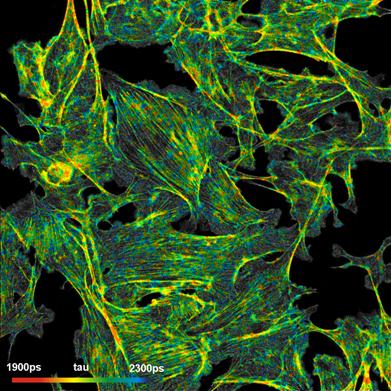
Fig. 4: FLIM
of a BPEA sample, 1024x1024 pixels, 1024 time channels, acquisition time 2
seconds. DCS-120 system with 488 nm diode laser and HPM-100-06 ultra-fast
hybrid detector.
An image of the same sample recorded with
an acquisition time of 10 seconds (5 frames of the scanner) is shown in Fig. 5.
The decay data in a 10x10 pixel spot and a decay curve integrated over the
entire image are shown in Fig. 6. The image and the decay curves show that the
system is able to record FLIM data of extraordinary quality within relatively
short acquisition times.
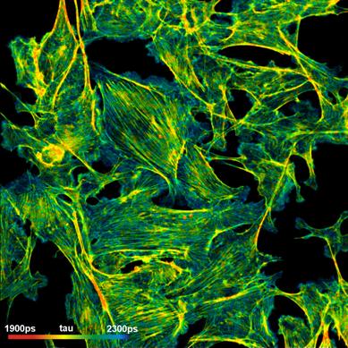
Fig. 5: FLIM
of a BPEA sample, 1024x1024 pixels, 1024 time channels, acquisition time 10
seconds. DCS-120 system with BDL-SMN 488 nm ps diode laser and HPM-100-06 ultra-fast
hybrid detector.
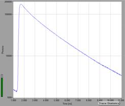
Fig. 6: Decay curves from the data shown in Fig. 5. Left: Decay data in a
10x10 pixel spot. Right: Decay curve from the entire image.
Time Resolution
The data shown in Fig. 4, Fig. 5, and Fig. 6
were recorded with an HPM-100-06 ultra-fast hybrid detector. With the bh
SPC-150N modules, this detector delivers an IRF of about 20 ps FWHM (full
width at half maximum) [1, 7]. The IRF width in Fig. 6 is about 60 ps, due
to the pulse width of the BDL-SMN 488 nm picosecond diode laser. The
question is how fast an IRF can be obtained with the Photon Spinner when a fast
laser is used.
Fig. 7, left, shows the electrical instrument
response functions of the four SPC 150N modules with the PHDIS-04 Photon
Spinner. Surprisingly, the IRF width of the individual modules is 6.7 to
6.9 ps, i.e. only insignificantly longer than the IRF of the modules
themselves (typically 6.6 ps).
Due to transit time differences in the
Photon Spinner and in the connecting cables the IRFs of the four TCSPC channels
appear slightly shifted, see Fig. 7, left. The shift can be corrected by using
separate TAC offsets for the individual TCSPC modules [1]. Fine alignment is
achieved by tweaking the Zero Cross levels of the CFDs of the modules.
Different Zero Cross shifts the trigger point up and down the leading edge of
the spinner output pulses, and thus acts as an extremely fine delay adjustment.
The variation in the Zero Cross has no influence on the IRF width because the
output pulses of the Photon Spinner have no amplitude jitter. The IRFs of the SPC-150N
modules after delay alignment are shown in Fig. 7, middle, the combined IRF of
the four modules is shown in Fig. 7, right. The combined IRF still has 6.8 ps
FWHM, much faster than the transit time spread of any commonly available photon
detector.
Fig. 7: Electrical IRFs of the four SPC-150N modules. Before (left) and
after delay alignment (middle). The combined IRF of the four SPC-150N is shown
on the right. The FWHM of the combined IRF is 6.8 ps.
The optical IRF of the entire system with
an HPM-100-06 detector is shown in Fig. 8. It was recorded with a Toptica Femto
Erb femtosecond fibre laser in the test setup described in [5].
Fig. 8: Instrument response function of an SPC-154N four-module package with
the Photon Spinner and an HPM‑100‑06 hybrid detector. FWHM is
22.6 ps.
Summary
The system described here is able to record
FLIM at high count rates and short acquisition times. Importantly, the system
reaches high count rate and short acquisition time without any reduction in
time resolution. FLIM data can still be recorded at sub-ps time channel with and
sub-25 ps IRF width (FWHM), thus fully exploiting the time resolution of the
bh TCSPC FLIM modules and ultra-fast hybrid detectors. It is therefore equally
suitable for fast FLIM and precision FLIM applications. The system can be used
in combination with the bh DCS-120 confocal and multiphoton scanning systems [12],
but also with laser scanning microscopes of other manufacturers [13, 14, 16, 15].
References
1.
W. Becker, The bh TCSPC handbook. Becker &
Hickl GmbH, 7th ed. (2017). Available on
www.becker-hickl.com
2.
W. Becker, Advanced time-correlated single
photon counting techniques. Springer, Berlin, Heidelberg, New York (2005)
3.
W. Becker (ed.), Advanced time-correlated single
photon counting applications. Springer, Berlin, Heidelberg, New York (2015)
4.
W. Becker, V. Shcheslavkiy, S. Frere, I. Slutsky, Spatially Resolved Recording of
Transient Fluorescence-Lifetime Effects by Line-Scanning TCSPC. Microsc. Res.
Techn. 77, 216-224 (2014)
5.
Becker & Hickl GmbH, Sub-20ps IRF Width from
Hybrid Detectors and MCP-PMTs. Application note, available on
www.becker-hickl.com
6.
Becker & Hickl GmbH, Ultra-fast HPM
Detectors Improve NAD(P)H FLIM. Application note, available on
www.becker-hickl.com
7.
W. Becker, A. Bergmann, C. Biskup, Multi-Spectral
Fluorescence Lifetime Imaging by TCSPC. Micr. Res. Tech. 70, 403-409 (2007)
8.
W. Becker, C. Junghans, A. Bergmann, Two-Photon
FLIM of Mushroom Spores Reveals Ultra-Fast Decay Component. Application note
(2021), available on www.becker-hickl.com.
9.
W. Becker, A. Bergmann, C. Junghans, Ultra-Fast
Fluorescence Decay in Natural Carotenoids. Application note, available on www.
becker-hickl.com
10.
Wolfgang Becker, Vladislav Shcheslavskiy, Vadim
Elagin, Ultra-Fast Fluorescence Decay in Malignant Melanoma. Application note,
available on www. becker-hickl.com
11.
Becker & Hickl GmbH, Simultaneous
Phosphorescence and Fluorescence Lifetime Imaging by Multi-Dimensional TCSPC and
Multi-Pulse Excitation. Application note, available on www.becker-hickl.com
12.
Becker & Hickl GmbH, DCS-120 Confocal
Scanning FLIM Systems. User handbook, 7th ed. (2017). Available on
www.becker-hickl.com
13.
Becker & Hickl GmbH, FLIM Systems for
Zeiss LSM 710 / 780 / 880 Family Laser Scanning Microscopes. User Handbook, 7th
ed. (2017). Available on www.becker-hickl.com
14.
Becker & Hickl GmbH, TCSPC FLIM Systems
for Nikon A1 Laser Scanning Microscopes. Data sheet, available on
www.becker-hickl.com.
15.
Becker & Hickl GmbH, Multiphoton FLIM
with the Leica HyD RLD Detectors. Application note, available on
www.becker-hickl.com
16.
Becker & Hickl GmbH, FLIM systems for
Laser Scanning Microscopes. Overview brochure (2017), available on
www.becker-hickl.com.
17.
Becker & Hickl GmbH, SPCM Software Runs
Online-FLIM at 10 Images per Second. Application note, available on
www.becker-hickl.com
18.
W. Becker, A. Bergmann, G. Biscotti, K. Koenig,
I. Riemann, L. Kelbauskas, C. Biskup, High-speed FLIM data acquisition by
time-correlated single photon counting, Proc. SPIE 5323, 27-35 (2004)
19.
V. Katsoulidou, A. Bergmann, W. Becker, How fast
can TCSPC FLIM be made? Proc. SPIE 6771, 67710B-1 to 67710B-7 (2007)
20.
X. Liu, D. Lin, W. Becker, J. Niu, B. Yu, L.
Liu, J. Qu, Fast fluorescence lifetime imaging techniques: A review on
challenge and development. Journal of Innovative Optical Health Sciences,
1930003-1 to -27 (2019)
Contact:
Wolfgang Becker
Becker & Hickl GmbH
Berlin, Germany
Email: becker@becker-hickl.com
