With Version 9.72 SPCM software the bh TCSPC FLIM systems and the DCS-120 Confocal and Multiphoton FLIM Systems record and display fluorescence lifetime images at a rate of 10 images per second. The calculation of the lifetime images is based on the first moment of the decay data in the pixels of the images. The first-moment technique combines short calculation times with near-ideal photon efficiency. It works for all SPC-QC-104, SPC-150, SPC-150N, SPC-160, and SPC-180N FLIM systems that use fast scanning. In combination with the preview mode of the SPCM software it can be used to select interesting cells within a larger sample for subsequent high-accuracy FLIM acquisition. In FLIM experiments with longer acquisition time it helps the user evaluate the signal-to-noise ratio of the data and decide whether enough photons have been recorded to reveal the expected lifetime effects in the sample.

Keywords: FLIM, Fast FLIM, Rapid FLIM, Online FLIM

Related Application Notes

Download PDF

SPCM Software Runs Online FLIM at 10 Images per Second

W. Becker, C. Junghans, Becker & Hickl GmbH

Abstract: Version 9.72 SPCM software of the bh TCSPC/FLIM systems displays fluorescence lifetime images at a rate of 10 images per second. The calculation of the lifetime images is based on the first moment of the decay data in the pixels of the images. The first-moment technique combines short calculation times with near-ideal photon efficiency. It works for all SPC-150, SPC-150N, SPC-160, and SPC-830 FLIM systems that use fast scanning. In combination with the preview mode of the SPCM software it can be used to select interesting cells within a larger sample for subsequent high-accuracy FLIM acquisition. In FLIM experiments with longer acquisition time it helps the user evaluate the signal-to-noise ratio of the data and decide whether enough photons have been recorded to reveal the expected lifetime effects in the sample.

Fast FLIM

Fast FLIM by TCSPC has been demonstrated on several occasions. Time-series FLIM by a record-and-save procedure has been described in [2], time-series FLIM by memory swapping in [3] and [11], temporal mosaic FLIM in [3] and [6], and triggered accumulation of time series for imaging Ca⁺⁺ transients in [3, 6, 7] and [9]. These techniques are aiming at the recording of fast dynamic effects in the fluorescence decay parameters, not at a fast sequential online display of lifetime images. Online display not only requires that the FLIM data are recorded within an extremely short acquisition time but also that the fluorescence lifetime is calculated from the decay data in a similarly short period of time. The task is complicated by the fact that the signal-to-noise ratio of a FLIM recording cannot be higher than

(1)

where N is the number of photons in the pixels. The number of photons available within a given period of time (the photon count rate) is limited by the sample itself: Excitation power or fluorophore concentration above a certain level cause invasive effects to the sample. Count rates obtained in FLIM experiments are thus rarely higher than a few MHz. The speed of online-FLIM is therefore limited by the decrease of the signal-to-noise ratio with increasing image rate. The requirements for fast online FLIM are therefore:

- The recording technique must record the photons in a way that the SNR comes close to the ideal value. That means the decay curve must be recorded in a sufficiently large number of time channels, with a negligible IRF width, and with negligible background from detector dark counts, detector afterpulsing, or daylight pickup [12]. TCSPC comes very close to the ideal conditions, and achieves a signal-to-noise ratio very close to the ideal value.

- the calculation algorithm for the lifetime must not only be fast enough to analyse the images within a time shorter than the image period but also extract the lifetime from the recorded data at the ideal signal-to-noise ratio inherent to the TCSPC data.

Fast Calculation of Lifetimes from TCSPC Data

Lifetime Calculation Algorithms

There is a number of fast algorithms for lifetime calculation from TCSPC data. The lifetime can be derived from the photon numbers in two time intervals (time gates), from the time until the integral of the decay curve reaches 1-1/e of the maximum, or from the phase and the amplitude at the fundamental frequency after transformation in the frequency domain. All these algorithms have their own problems: Time-interval analysis delivers systematic errors if the rise of the fluorescence does not coincide with the beginning of the first time interval, or a sub-optimal SNR if the fluorescence rises before the first time interval. Moreover, the width of the time gates must be adjusted to the expected lifetime, which is possible only if the approximate lifetime is known. The lifetime determination via the integral does not use all photons, and is influenced by the uncertainty of the 1-1/e point of the integral. The SNR is thus sub-optimal. The SNR of frequency domain analysis is sub-optimal if only the phase and amplitude at the fundamental frequency are considered (the photons are weighted differently depending on their time in the decay curve). Sub-optimal SNR is, however, compensated by the ability to automatically combine pixels of similar phase/amplitude signature. The result is a phasor plot, not a lifetime image. It therefore does not immediately match the requirements of online FLIM.

First-Moment Algorithm

An almost ideal SNR from TCSPC data is obtained by calculating the lifetime via the first moment of the decay data [8]. The method has been suggested first by Z. Bay in 1950 for the determination of excited nuclear state lifetimes in coincidence experiments [1]. The first moment of a photon distribution is

(2)

with N = total number of photons, t = time of individual time channels, n(t) = photon number in individual time channels

The first moment can also be considered the average arrival time of all photons in the decay curve. For a single-exponential decay, it can easily be shown that the first moment delivers an ideal SNR: The standard deviation of the photon arrival time is t, and the standard deviation of the average arrival time of a large number of photons is . The relative standard deviation, or the SNR, is thus , and the signal-to-noise ratio is .

The fluorescence lifetime (of a single-exponential decay approximation) is the difference of the first moment of the fluorescence and the first moment of the IRF:

(3)

The relations are illustrated graphically in Fig. 1. The blue dots are the photon numbers in the time channels of the pixel, the green curve is the IRF. M1 of Fluorescence is the first moment calculated according to (2), M1 of IRF is the M1 of the IRF calculated by the same formula. Tau is the fluorescence lifetime calculated according to (3). The red curve is the convolution of a single-exponential function, f(t) = e^-t/^t, with the IRF.

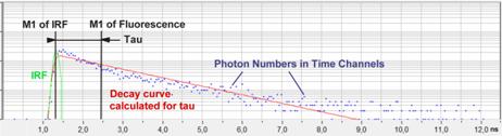
Fig. 1: First-moment calculation of fluorescence lifetime. The lifetime is the difference of the first moment of the fluorescence and the first moment of the IRF.

For a double-exponential decay, it can be shown that (3) delivers the intensity-weighted average of the lifetimes of the two components. The signal-to-noise ratio remains very close to for a wide range of lifetime and intensity ratios of the components.

To obtain correct lifetimes the first moment of the IRF has to be known. This is no problem for TCSPC FLIM. M1_IRF can be obtained either by analysing a FLIM data file with SPCImage [3], or from decay data of a fluorophore with known lifetime. In any case, the IRF can be recorded with a high N, its uncertainty therefore does not significantly contribute to the uncertainty of t.

Other requirements for the M1 calculation of lifetimes are that the background of the decay signal is negligible, and that the entire decay curve is recorded up to a time channel beyond which no more photons are recorded. Also this is no problem for fast online display. Due to the short acquisition time, background is low or even not detectable, and the decay function drops quickly to the point where later photons are unlikely to be detected. Examples can be seen in Fig. 2 and Fig. 3, middle.

Binning of Decay Data

Online FLIM at image rates faster than one image per second delivers very low photon numbers in the pixels. An example is shown in Fig. 2. The decay curve (shown left) is from a single pixel of a FLIM recording of 256x256 pixels, recorded at an acquisition time of 0.2 seconds (5 frames per second). The entire curve contains about 45 photons. The corresponding FLIM image is shown in Fig. 2, right. According to (1) the SNR of the fluorescence lifetime in the bright pixels of the image is about 7. The noise in the lifetime can easily be seen in Fig. 2.

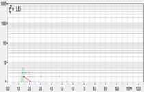
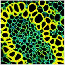
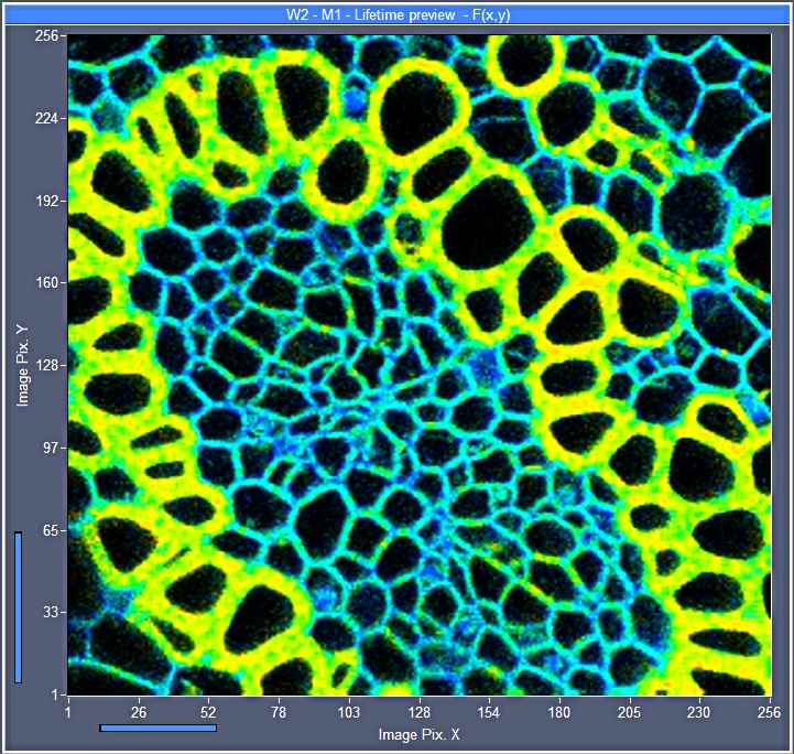
Fig. 2: Online FLIM with acquisition time 0.2 seconds (5 frames/second). 256x256 pixels, no binning. Left: Decay curve in brightest pixel, the photons are barely visible between t = 1ns ... 2ns. Right: Lifetime image calculated by M1 algorithm, red to blue = 1000 to 3000 ps.

A substantial improvement is obtained by binning the decay data for the lifetime analysis. The binning algorithm used in SPCM is the same as in SPCImage. For every pixel of the image, it uses not only the photons in this pixel but also the photons in the pixels around, see Fig. 3, left. On average, this yields a photon number 9 times larger than without binning (Fig. 3, middle), and a 3 times better SNR of the lifetime. The lifetime image is built up from the intensity data of the unbinned pixels and the lifetime data from the binned pixels. The image calculated this way is shown in Fig. 3, right.

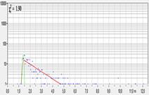
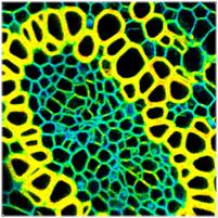
Fig. 3: Online FLIM, parameters same as Fig. 2, but with binning of lifetime data, 3x3 pixels. Left: Decay curve in brightest pixel. Right: Lifetime image calculated by M1 algorithm, red to blue = 1000 to 3000 ps.

The improvement in image quality is striking: The noise in the lifetime is much lower, but, surprisingly, there is no apparent reduction in image definition. This has two reasons. The first one is the way the human eye-brain combination processes images. Perception of image definition comes exclusively from the intensity, the colour is just an overlay on the intensity image. Since the intensity data have not been binned the apparent definition is not impaired by binning. The second one is the way images are recorded in microscopy. Usually, the images are oversampled, i.e. the Airy disc (or point-spread function) is imaged on an area of several pixels. Binning has, of course, little effect on data which are already smoothed by spatial convolution with the Airy disc.

Implementation in the SPCM Software

The Online-Lifetime display function is implemented in the SPCM software, version 9.72 or later. To activate the online display, open the 3D Trace Parameter panel and define a display window for Lifetime Preview data, see Fig. 4, left.

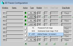
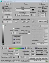
Fig. 4: SPCM Definitions for online lifetime display

The pseudo-colour range for the lifetime display is defined in the Display Parameter panel corresponding to the selected display window. The display parameters also have sliders for brightness and contrast. The sliders work independently of the scale definitions in the upper part of the display parameters, they are also available when autoscale is selected.

As described above, the first-moment calculation needs the first moment of the IRF. This can either be typed in or calculated from a FLIM data file. In the first case, the moment of the IRF can be taken from the SPCImage data analysis software. Load a FLIM file into SPCImage, select Model, 1st Moment, and find the 1st Moment of IRF in the lower right part of the SPCImage panel. The file can be from any sample. It is only important that it was recorded by the same FLIM system, with similar optical and electrical path length, and with similar TAC parameters as the data to be displayed.

In the second case SPCM uses a FLIM data file from a reference sample. This sample should have a uniform lifetime, and the lifetime must be known or determined with SPCImage. The file must, of course, be recorded with the same instrument configuration, and with the same TAC parameters that are used for the online display. For diode-laser excitation, it is recommended to use also the same (electrical) laser power. If you need different laser power, change the power optically [3, 4]. It is not necessary to record a new reference file every day. The bh TCSPC modules have an extremely good timing stability [3]. The reference data therefore remain valid over weeks or months.

To use the online lifetime display for FLIM at high image rate the Repeat function of the SPCM software in combination with a short Collection Time and a short Repeat Time is used. For frequent updates of the FLIM display during a measurement with long acquisition time the desired update interval is defined by Display Time. The parameters are accessible in the lower left part of the SPCM main window. For details please see The bh TCSPC Handbook [3] or handbooks of the DCS-120 system [4] or of the FLIM systems for the Zeiss laser scanning microscopes [5].

Typical Results

Online lifetime images recorded at a rate up to 10 images per second (acquisition time 100 ms) are shown in Fig. 5 through Fig. 7. The images were recorded by a bh DCS-120 confocal scanning system [4]. A convallaria sample was used as a test object, the excitation wavelength was 488 nm. The count rates were in the range of 1 to 2 MHz, averaged over the entire image. The data were recorded with 256 time channels and a time channel width of 49 ps. All images are displayed with the same lifetime scale, 1000 ps (red) to 3000 ps (blue).

Fig. 5 shows 128x128-pixel images recorded with acquisition times of 0.1 s, 0.5 s, and 2 s. The upper row shows images without binning, the lower row images with 3x3 pixel binning of the decay data. The images show that lifetime images of reasonable quality are obtained even at an acquisition time of 100 ms, or an image rate of 10 per second.

Good images at a resolution of 256x256 pixels and 512x512 pixels were obtained at about 5 images and 2 images per second, respectively (Fig. 6 and Fig. 7). Also here, binning reduces the lifetime noise substantially without causing noticeable blur of the images.

With 64-bit SPCM software, the image size can be increased to 1024x1024 pixels and more [3, 4, 14]. The M1 algorithm is fast enough to process such data in a fraction of a second. Images of reasonable lifetime resolution are obtained down to an acquisition time of 2 seconds, or an image rate of 0.5 per second. An example is shown in Fig. 8

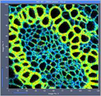
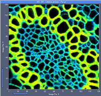
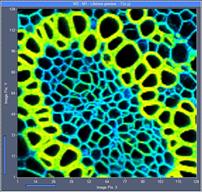
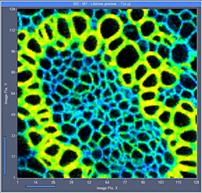
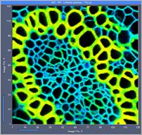
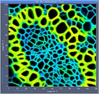
Fig. 5: 128x128-pixel images. Acquisition time 0.1s, 0.5s, 2s. Upper row: No binning. Lower row: Binning 3x3 pixels

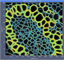
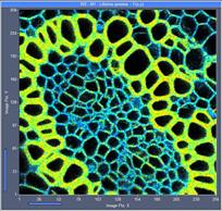
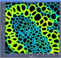
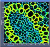
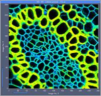
Fig. 6: 256x256-pixel images. Acquisition time 0.2s, 0.5s, 2s. Upper row: No binning. Lower row: Binning 3x3 pixels

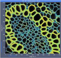
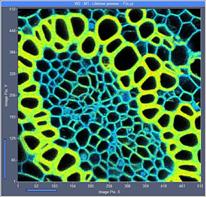
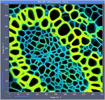
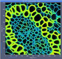
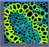
Fig. 7: 512x512-pixel images. Acquisition time 0.5s, 2s, 5s. Upper row: No binning. Lower row: Binning 3x3 pixels

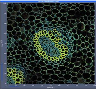
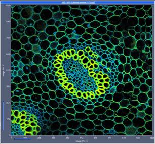
Fig. 8: 1024x1024-pixel image, acquisition time 2 seconds. Left without, right with 3x3 pixel binning of the decay data.

Discussion

The results shown above demonstrate that fast online FLIM is feasible almost up to the maximum frame rate of the commonly used galvanometer scanners. It should be taken into account, however, that the examples shown here were recorded with a convallaria sample. In this sample, the lifetime varies over a range of about 1:2.5. In real-world FLIM samples the lifetime variation is often smaller. Selecting FRET-positive cells in a culture of donor-and-acceptor expressing cells requires a lifetime resolution of about 1:1.25. Obtaining images of similar quality as for the convallaria would require four times the photon number, and thus four times the acquisition time, see (1). This would be about 0.4 seconds for a 128x128 pixel image with binning. This is still an acceptable image rate. Even in clinical FLIM applications, with metabolism-induced lifetime changes on the order of 1:1.1 [10, 13] images can probably be displayed at rates faster than one image per second.

References

1. Z. Bay, Calculation of decay times from coincidence experiments. Phys.
Rev. 77, 419 (1950)
2. W. Becker, Advanced time-correlated single-photon counting techniques. Springer,
Berlin, Heidelberg, New York, 2005
3. W. Becker, The bh TCSPC handbook. 6th edition, Becker & Hickl
GmbH (2015), available on www.becker-hickl.com
4. Becker & Hickl GmbH, DCS-120 Confocal Scanning FLIM Systems, 6th
ed. (2015), user handbook. www.becker-hickl.com
5. Becker & Hickl GmbH, Modular FLIM systems for Zeiss
LSM 710 / 780 / 880 family laser scanning microscopes. 6th ed. (2015),
user handbook. available on www.becker-hickl.com
6.
W. Becker, V. Shcheslavskiy, H. Studier, TCSPC FLIM with Different
Optical Scanning Techniques, in W. Becker (ed.) Advanced time-correlated single
photon counting applications. Springer, Berlin, Heidelberg, New York (2015)
7.
W. Becker, V. Shcheslavkiy, S. Frere, I. Slutsky,
Spatially Resolved Recording of Transient Fluorescence-Lifetime Effects by
Line-Scanning TCSPC. Microsc. Res. Techn. 77, 216-224 (2014)
8. I. Isenberg, R.D. Dyson, The analysis of fluorescence decay by a
method of moments. Biophys. J. 9, 1337-1350 (1969)
9.
S. Frere, I. Slutsky,
Calcium imaging using Transient Fluorescence-Lifetime Imaging
by Line-Scanning TCSPC. In: W. Becker (ed.) Advanced time-correlated single
10. S. Kalinina, V. Shcheslavskiy, W. Becker, J. Breymayer, P. Schäfer,
A. Rück, Correlative NAD(P)H-FLIM and oxygen sensing-PLIM for metabolic mapping.
J. Biophotonics (2016)
11. V. Katsoulidou, A. Bergmann, W. Becker, How fast can TCSPC FLIM be
made? Proc. SPIE 6771, 67710B-1 to 67710B-7 (2007)
12. M. Köllner, J. Wolfrum, How many photons are necessary for
fluorescence-lifetime measurements?, Phys. Chem. Lett. 200, 199-204 (1992)
13. W. Y. Sanchez, M. Pastore, I. Haridass, K. König, W. Becker, M. S.
Roberts, Fluorescence Lifetime Imaging of the Skin. In: W.
Becker (ed.) Advanced time-correlated single photon counting applications.
Springer, Berlin, Heidelberg, New York (2015)
14. H.
Studier, W. Becker, Megapixel FLIM. Proc. SPIE 8948 (2014)
Contact:
Wolfgang Becker
Becker & Hickl GmbH
Berlin, Germany
Email: becker@becker-hickl.com