This application note reviews the options of fast-acquisition TCSPC FLIM. We describe the parameters which limit the acquisition speed, both in the sample and in the recording system. We show that a standard bh FLIM system is able to record and display FLIM images at a rate much higher rate than commonly believed. We describe how faster acquisition times and faster image rates are obtained in the bh FASTAC FLIM system. Moreover, we show how fast dynamic changes in the fluorescence behaviour of a sample can be recorded under conditions where the sample does not deliver the count rate required for fast-acquisition FLIM.

Keywords: Fast FLIM, Rapid FLIM, Pile-Up, Triggered Accumulation, Temporal Mosaic FLIM

Related Application Notes

Download PDF

Fast-Acquisition TCSPC FLIM: What are the Options?

Wolfgang Becker, Stefan Smietana, Becker & Hickl GmbH, Berlin, Germany

Abstract: This application note reviews the options of fast-acquisition TCSPC FLIM. We describe the parameters which limit the acquisition speed, both in the sample and in the recording system. We show that a standard bh FLIM system is able to record and display FLIM images at a rate much higher rate than commonly believed. We describe how faster acquisition times and faster image rates are obtained in the bh FASTAC FLIM system. Moreover, we show how fast dynamic changes in the fluorescence behaviour of a sample can be recorded under conditions where the sample does not deliver the count rate required for fast-acquisition FLIM.

General Considerations on Fast FLIM Acquisition

There is currently a run towards faster and faster acquisition in fluorescence lifetime imaging (FLIM). Unfortunately, these developments usually ignore the fact that, in most instances, the limitations are in the sample rather than in the recording electronics. The fastest recording system cannot record fast if the sample is not able to deliver the photons needed to acquire the data at this speed. Moreover, recording speed is usually obtained on the expense of time resolution or data complexity, such the capability to record a fully resolved fluorescence decay function in each pixel. These are exactly the features needed in typical FLIM applications, such as metabolic imaging, protein interaction experiments, and other molecular imaging applications. Ignoring these needs by just recording a lifetime in the pixels of the image means reducing the fluorescence decay function to a simple contrast parameter. In other words, Fast FLIM sacrifices the most important features of FLIM for a single parameter (recording speed) which, ironically, cannot be exploited in the typical applications. This application note describes the parameters that determine the speed of FLIM recording, and shows the way to record FLIM at short acquisition time without compromises in time resolution or data complexity.

What Limits the Acquisition Speed of FLIM?

Signal-to-noise ratio

The signal-to-noise ratio (SNR) of FLIM depends on the number of photons per pixel. Ideally, the SNR of the fluorescence lifetime, t, is

with N = number of photons per pixel. For a given photon rate obtained from the sample the number of photons, N, decreases with decreasing acquisition time, and so does the signal-to-noise ratio of the lifetime data.

The sample must feed the recording system with enough photons

The fastest FLIM system does not yield images within a short acquisition time if the sample does not deliver the required photon rate. For example, to record a 256 x 256 pixel image with an SNR of 10 (or 10% standard deviation) 6.5 million photons are required. To record the data within 1 second the photon rate must be 6.5×10⁶ s^-1. To record a 512 x 512 pixel image at the same accuracy and acquisition time a photon rate of 25×10⁶s^‑1 would be required. Photon rates this high can only be obtained from strongly stained samples, such as the often used convallaria sample (stained with acridin orange) or mouse kidney samples (stained with Alexa dyes). Samples used in FLIM experiments normally contain far lower fluorophore concentrations and thus deliver lower count rates. NADH in live cells yields no more than about 200,000 photons per second, and fluorescent proteins in FRET experiments no more than 500,000. Simultaneously, the requirements to the SNR are higher - lifetime variations on the order of 2% have to be detected, and multi-exponential decay analysis must be performed. Under these conditions, the required photon numbers cannot be obtained within one or two seconds.

Photobleaching and photodamage

Attempts to increase the count rate by increasing the excitation power induce lifetime changes in the sample, impair the viability of the cells, or destroy the sample altogether. Fig. 1 shows two examples. The left image shows a convallaria sample, the central region of which has been scanned with a 405-nm laser for 1 minute at a laser power of 0.5 mW. The right image shows an NADH image of live cells. It was obtained with two-photon excitation at 5% of the available laser power. The average count rate over the entire image was 350,000 s^-1. Within 20 seconds, the irradiation caused damage in form of bright spots of extremely short lifetime.

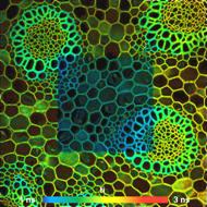
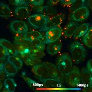
Fig. 1: Left: Convallaria image, region in the centre scanned with 405 nm laser. Right: Two-photon NADH image of live cells. In the bright red spots photodamage has occurred, revealing itself by an ultra-fast decay component.

It should be noted that photobleaching not only has an impact on the imaging process, it also produces radicals. Radicals cause photochemical stress to the cells. Attempts to reduce photobleaching by increasing the fluorophore concentration do not reduce the amount of radicals produced. The absolute amount of converted fluorophore remains the same, and so does the photochemical stress to the cells.

Assuming we get enough photons: How fast can TCSPC FLIM record?

TCSPC FLIM has a number of fascinating features. It delivers an excellent time resolution [8, 9] and a near-ideal photon efficiency [1, 2], it has multi-exponential decay-recording capability, is able to record complex data in a multi-parameter space [1, 2, 3], and simultaneously records FLIM and PLIM [6, 7]. These features are the basis of metabolic FLIM, FLIM-FRET, multi-parameter and multi-wavelength FLIM, and functional FLIM [3]. Should we sacrifice these functions and applications for just faster acquisition - a feature which can be used only for a minority of samples and a minority of experiments? No. Instead, we should find a way o record at high photon rates while maintaining the superior functionality of TCSPC FLIM.

How fast is a normal TCSPC FLIM system?

The Pile-Up Effect

As the speed-limiting effect of TCSPC FLIM usually the Pile-Up is considered. Pile-up is the possible detection (and loss) of a second photon in the same excitation pulse period with a previous one [1, 2]. The probability of pile-up increases with increasing count rate. It causes a distortion of the recorded decay curves, and a shift of the measured decay times towards lower values, see Fig. 2.

Fig. 2: The pile-up effect. A second photon in the same pulse period with a previous one is lost. The result is a distortion of the measured decay profile.

It is commonly believed that the photon rate must be lower than 0.1% of the pulse repetition rate, f_rep, to avoid pile-up distortion. This is wrong. The Pile-Up Limit of 0.1% probably stems from a typo in the early TCSPC literature. Correct is that the photon rate can be as high as 10% (or 0.1 × f_rep) without causing more than 5% of error in the recorded lifetimes [1, 2]. This is 100 times more than commonly believed!

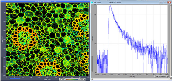
Consequently, a standard TCSPC FLIM system can record considerably faster than most users expect. Depending on the expectations to the lifetime accuracy and on the number of pixels of the image acquisition times between a few seconds and a few 100 ms can be achieved [10]. Fig. 3 shows two examples. The left image (256 x 256 pixels) was obtained within 0.2 seconds, the right image (512 x 512 pixels) within 2 seconds.

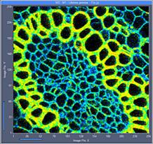
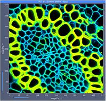
Fig. 3: Fast acquisition with standard SPC-150 FLIM system. Left: 256 x 256 pixels, acquisition time 0.2 seconds. Right: 512 x 512 pixels, acquisition time 2 seconds. DCS-120 FLIM system, online-lifetime display by SPCM software.

The pile-up free photon rate can be increased by using several detectors and TCSPC modules in parallel and combining the signals of the modules. Parallel-channel FLIM has been demonstrated for two channels [19], four channels [18], and 8 channels [17]. Most bh FLIM system already have two or four detectors and TCSPC channels [1, 14, 15, 16]. These parallel channels can easily by used to run fast FLIM on these systems. Online combination of the channels has been implemented in SPCM, version 9.78 [13].

The bh FASTAC FLIM System

The bh FASTAC FLIM system uses one detector and four TCSPC modules. The photon pulses from the detector are distributed into the TCSPC modules by a module called Photon Spinner [11]. The principle is shown in Fig. 4. As usual, the photon pulses from the detector are passing a constant-fraction discriminator, CFD. The output pulses of the CFD have a constant width and a time independent of the pulse amplitude of the detector pulses [1]. The pulses from the CFD control a four-way switch that distributes the pulses to four TCSPC modules. Every photon pulse from the CFD rotates the switch by one position. The trick of the solution is that every photon sets the switch not for the next photon, but for itself. To do so, the photon pulses pass a delay line. Every photon arrives at the switch a short time after the switching action has been completed. This way, the Photon Spinner avoids the influence of possible switching transients on the timing: Because every photon pulse arrives at the switch at a fixed time after the switching action the sum of the photon pulse and the switching transient is the same for all photons. It is also independent of the time of the photon in the laser pulse period. Therefore, the time resolution (IRF width) of the system and the differential nonlinearity of a bh FASTAC system is the same as for a single-module system [11].

Fig. 4: Principle of the bh FASTAC FLIM system

Fig. 5: FLIM recorded by the bh FASTAC system. Left: 512 x 512 pixel image, recorded within 0.5 seconds. Right: Decay function from a 10x10 pixel area in the centre of the image. DCS-120 confocal FLIM system. Image and decay curve displayed by online FLIM functions of SPCM.

Faster than Fast FLIM - Temporal Mosaic Recording with Triggered Accumulation

What if the sample does not deliver the photons for fast FLIM? In that case a fast FLIM system - no matter whether it is a parallel-detector system or a FASTAC system - will deliver a similar image as a standard single-channel system. Can we detect fast changes in the fluorescence decay behaviour of a sample under these conditions? Surprisingly, the answer is yes.

The way to do so is Temporal Mosaic FLIM. Consider a sample in which, by some external stimulation, a lifetime change is induced. Assume that the FLIM system records a series of FLIM images into subsequent elements of a large data array (a mosaic of FLIM data) [1]. If the recording starts with the stimulation, the result will be a fast time-series of FLIM recordings. If each image is recorded in just one frame the series will be as fast as the scanner can go.

Now, lets further assume that the stimulation is applied to the sample periodically. What will happen? With every stimulation the recording will run through all elements of the data array, and the data will be accumulated. This is the idea of Temporal Mosaic FLIM with Triggered Accumulation [1, 3, 5]. The result is a fast time series the signal-to-noise ratio of which does no longer depend on the speed of the series. For a given photon rate, it only depends on the total acquisition time.

The principle is illustrated in Fig. 6. In fact, the FLIM system records a photon distribution over the scan coordinates, the times of the photons after the excitation pulses, and the times of the photons after the stimulation.

Fig. 6: Principle of Temporal Mosaic FLIM with Triggered Accumulation

A FLIM recording of the Calcium²⁺ transient in live neurons is shown in Fig. 7. The data were recorded with a Zeiss LSM 7 multiphoton microscope in combination with a bh Simple Tau 150 (SPC-150) FLIM system [1, 5]. The time per image element was 38 ms.

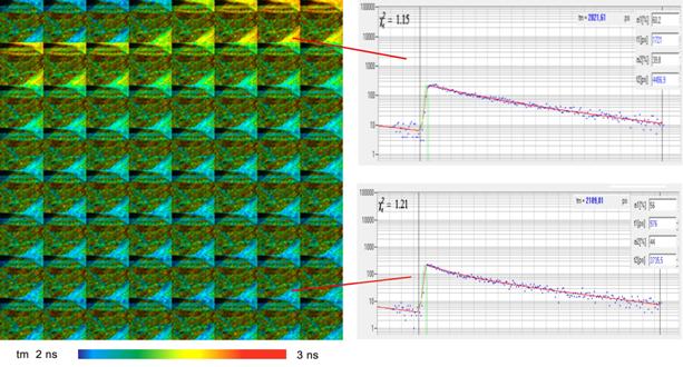
Fig. 7: Calcium²⁺ transient in live neurons. Zeiss LSM 7MP, SPC-150 FLIM module. Time per image element 38 ms, 100 stimulation periods accumulated.

Resolving Transient Effects by Line-Scanning TCSPC

In a temporal mosaic recording as the one shown in Fig. 7 the speed is limited by the minimum frame time of the scanner. Faster sequences can be obtained by resonance scanners or by line scanning. A typical galvanometer scanner can scan one line in about 1 to 2 milliseconds. The FLIM system then builds up a photon distribution over the distance along the line, the times of the photons after the excitation pulses, and the time after the stimulation [4, 5]. An example is shown in Fig. 8. The time resolution within the stimulation period is 2 ms.

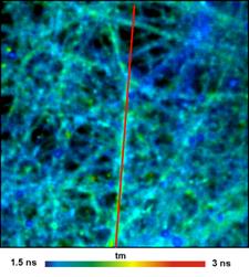
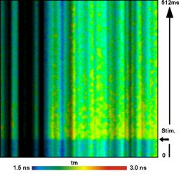
Fig. 8: Recording transient lifetime effects by line scanning TCSPC. Left: FLIM image of the sample, with selection of line scan within the sample. Right: Line-scanning data, horizontal distance along the line, vertical time after stimulation, colour fluorescence lifetime of Ca²⁺ sensor.

Summary

The recording speed of TCSPC FLIM is by one part limited by the capability of the sample to deliver high photon rates, by another part by the capability of the FLIM system to record this rate without loss of photons and without distortion of the recorded decay profiles. The limiting effect of the sample on the acquisition speed is usually underestimated, whereas the limitations in the recording system are over-estimated. Samples for molecular imaging experiments - the most widespread application of FLIM - do not deliver the count rates required for fast-acquisition FLIM. Of the recording side, TCSPC FLIM can record images surprisingly fast. In particular, the much-feared pile-up effect is far less a speed limitation than commonly believed.

As a consequence, standard TCSPC FLIM systems are well capable of recording at the maximum photon rate typical FLIM samples deliver. Nevertheless, there are samples which can deliver photon rates beyond the capabilities of a normal TCSPC FLIM system. To exploit the count rates from these samples for increasing the recording speed two solutions are possible.

The signals can be split into several channels optically, and recorded by several TCSPC modules in parallel. The solution is simple and can be used in any bh FLIM system that has several parallel TCSPC channels. All that is needed is a beamsplitter for the optical signals to the detectors.

Fast acquisition with a single detector is achieved by the bh FASTAC fast-acquisition FLIM system. The FASTAC system distributes the photon pulses of one detector into four TCSPC channels electronically.

These fast FLIM principles achieve short acquisition times without compromises in time resolution (IRF width), number of time channels, or multi-dimensional recording capabilities of TCSPC FLIM. They do, however, require a sample that deliver extremely high count rates. For samples which do not deliver the required count rates a fast FLIM system is no faster than a standard single-channel system.

Recording of fast changes in the fluorescence behaviour under sample-limited (low-count rate) conditions can be achieved by temporal mosaic FLIM with triggered accumulation. Different than parallel-channel or FASTAC FLIM this technique does not require high count rates from the sample.

References

1. W. Becker, The bh TCSPC handbook. Becker & Hickl GmbH, 9th ed. (2021). Available on www.becker-hickl.com

2. W. Becker, Advanced time-correlated single photon counting techniques. Springer, Berlin, Heidelberg, New York (2005)

3. W. Becker (ed.), Advanced time-correlated single photon counting applications. Springer, Berlin, Heidelberg, New York (2015)

4. W. Becker, V. Shcheslavkiy, S. Frere, I. Slutsky, Spatially Resolved Recording of Transient Fluorescence-Lifetime Effects by Line-Scanning TCSPC. Microsc. Res. Techn. 77, 216-224 (2014)

5. W. Becker, S. Frere, I. Slutsky, Recording Ca⁺⁺ Transients in Neurons by TCSPC FLIM. In:F.-J. Kao, G. Keiser, A. Gogoi, (eds.), Advanced optical methods of brain imaging. Springer (2019)

6. Becker & Hickl GmbH, Simultaneous Phosphorescence and Fluorescence Lifetime Imaging by Multi-Dimensional TCSPC and Multi-Pulse Excitation. Application note, available on www.becker-hickl.com

7. W. Becker, V. Shcheslavskiy, A. Rück, Simultaneous phosphorescence and fluorescence lifetime imaging by multi-dimensional TCSPC and multi-pulse excitation. In: R. I. Dmitriev (ed.), Multi-parameteric live cell microscopy of 3D tissue models. Springer (2017)

8. Becker & Hickl GmbH, Sub-20ps IRF Width from Hybrid Detectors and MCP-PMTs. Application note, available on www.becker-hickl.com

9. Becker & Hickl GmbH, Ultra-fast HPM Detectors Improve NAD(P)H FLIM. Application note, available on www.becker-hickl.com

10. Becker & Hickl GmbH, SPCM Software Runs Online-FLIM at 10 Images per Second. Application note, available on www.becker-hickl.com

11. Becker & Hickl GmbH, Fast-Acquisition TCSPC FLIM System with sub-25 ps IRF Width. Application note, available on www.becker-hickl.com

12. Becker & Hickl GmbH, Fast-Acquisition Multiphoton FLIM with the Zeiss LSM 880 NLO. Application note, available on www.becker-hickl.com

13. Becker & Hickl GmbH, New SPCM Version 9.80 Comes With New Software Functions. Application note, available on www.becker-hickl.com

14. Becker & Hickl GmbH, DCS-120 Confocal Scanning FLIM Systems. User handbook, 7th ed. (2017). Available on www.becker-hickl.com

15. Becker & Hickl GmbH, FLIM Systems for Zeiss LSM 710 / 780 / 880 Family Laser Scanning Microscopes. User Handbook, 7th ed. (2017). Available on www.becker-hickl.com

16. Becker & Hickl GmbH, FLIM systems for Laser Scanning Microscopes. Overview brochure (2017), available on www.becker-hickl.com.

17. Becker & Hickl GmbH, An 8-Channel Parallel Multispectral TCSPC FLIM System. Application note, available on www.becker-hickl.com