We demonstrate precision lifetime analysis on FLIM data of a moving object. The technique is based on temporal-mosaic recording and image segmentation by the phasor plot of bh SPCImage NG data analysis software. A cluster of phasors is selected in the phasor space, identifying pixels of a given decay signature in the FLIM mosaic. These pixels are back-annotated in the mosaic, selecting parts of the objects irrespectively of their location in the individual images. The decay data of the pixels within the selected areas are summed up. The result is a single decay curve with extremely high pixel number which can be analysed at high precision.

Keywords: FLIM, Moving Object, Phasor Plot, Image Segmentation

Related Application Notes

Download PDF

Precision Fluorescence-Lifetime Imaging of a Moving Object

Wolfgang Becker, Axel Bergmann, Becker & Hickl GmbH, Berlin, Germany

Abstract: We demonstrate precision lifetime analysis on FLIM data of a moving object. The technique is based on temporal-mosaic recording and image segmentation by the phasor plot of bh SPCImage NG data analysis software. A cluster of phasors is selected in the phasor space, identifying pixels of a given decay signature in the FLIM mosaic. These pixels are back-annotated in the mosaic, selecting parts of the objects irrespectively of their location in the individual images. The decay data of the pixels within the selected areas are summed up. The result is a single decay curve with extremely high pixel number which can be analysed at high precision.

The Problem

The recording of fluorescence-lifetime images of live objects is often impaired by motion in the sample. In cells motion can be induced by moving mitochondria, in animals by heart beat or simply by muscle activity. An example is shown in Fig. 1. It shows autofluorescence images of the leg of a water flee. The insect is squeezed between the slide and the cover slip. It moved the leg as it tries to escape. The images were recorded by TCSPC FLIM [1] with a bh DCS-120 confocal FLIM system at 470 nm excitation wavelength [2]. The image format is 256 x 256 pixels, 256 time channels. The images were recorded in single frames of 0.5 seconds. Despite the fast scan time the images are impaired by motion artefacts. The image on the right is even badly distorted as motion occurred during the scan time.

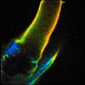
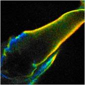
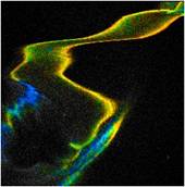
Fig. 1: Three images of a water flee, recorded with 0.5 s frame time. Lifetime images, generated by SPCImage NG. MLE fit, double-exponential model, mean (amplitude weighted) lifetime, binning 5 x 5 pixels.

The photon number in the individual pixels ranges from about from about 3 to 30. Such low photon numbers are typical of autofluorescence images. Even with binning of 5 x 5 pixels a reasonable lifetime is obtained only in the bright pixels. It is therefore desirable to increase the numbers of photons for the lifetime analysis. However, accumulating the images over a longer period of time is no option because motion would render the images useless. Higher count rate (by higher excitation power) is not applicable as well because it would damage the object under investigation within less than a minute. For the same reason, application of a 'fast FLIM' technique is no solution. The limitation is in the photon rate obtained from the sample, not in the counting capability of the FLIM system. Under these conditions a 'fast' FLIM technique is no faster than 'normal' TCSPC FLIM [3].

The Solution: Temporal Mosaic FLIM

Mosaic FLIM was originally introduced in the bh FLIM systems to record FLIM of large sample areas by sample stepping [1]. When used without sample stepping, the technique simply records a mosaic of time-series images [1]. An example for the water flee is shown in Fig. 2.

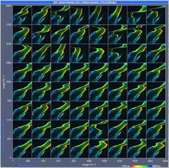
Fig. 2: Temporal Mosaic FLIM of a water flee. 64 images, each image recorded in a single frame of 0.5 seconds. Images 256 x 256 pixels, 256 time channels, lifetime display of bh SPCM data acquisition software.

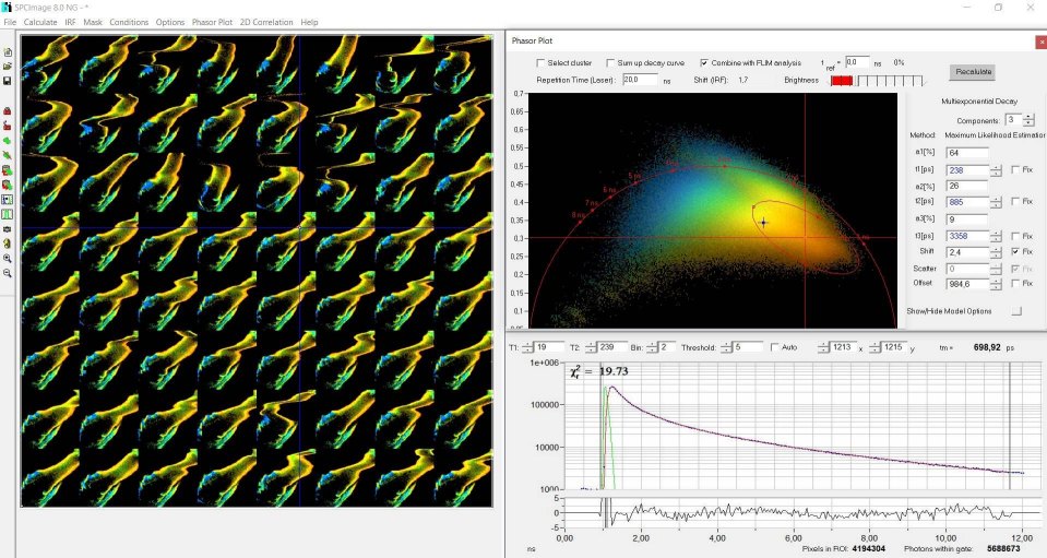
Data Processing by Phasor Image Segmentation

As expected, the individual images of the mosaic are no better than the ones shown in Fig. 1. However, there is a difference to a conventional time series. The FLIM mosaic is not a sequence of individual FLIM data sets but a single photon distribution. It can therefore be loaded into SPCImage data analysis software like a single image and analysed the usual way [1, 5], see Fig. 3. It is then possible to calculate a phasor plot over the entire mosaic. The result is shown in Fig. 4. The phasor plot shows the pixels of the image (in this case the mosaic) in an amplitude-phase diagram (the phasor space). The position in this diagram depends on the temporal shape of the decay data, not on the position in the image. A cluster of pixels selected in the phasor plot (ellipse in Fig. 4) therefore contains pixels of similar decay signature - irrespectively of their location in the image [1, 2].

Because the location in the phasor space does not depend on the location in the image it also does not depend on possible motion between the individual mosaic elements. The selection made in Fig. 4 selects pixels appearing orange in the FLIM image. Back annotation of the selected pixels in the mosaic therefore selects the leg of the water flee, see Fig. 5. A combination of the decay data of the selected pixels in a single decay curve is shown in Fig. 5, lower right. This curve contains more than 500 million photons. It can thus be analysed at high precision. The decay parameters obtained from a triple-exponential fit are shown in Fig. 5, upper right. A similar result for the blue pixels of the image is shown in Fig. 6.

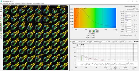
Fig. 3: Temporal-FLIM Mosaic data loaded into SPCImage NG.

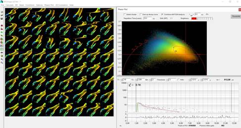
Fig. 4: Temporal-FLIM Mosaic loaded into SPCImage NG, Phasor Plot activated

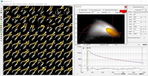
Fig. 5: Selection of orange pixels, back-annotation in the mosaic, and combination into a single decay curve

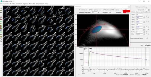
Fig. 6: Selection of blue pixels, back-annotation in the mosaic, and combination into a single decay curve

Summary

Precision lifetime analysis on a moving object is possible by recording a temporal mosaic of single frames, and selecting clusters of a given decay signature in the phasor plot of SPCImage NG. Pixels within the selected cluster represent parts of the object irrespectively of their location in the individual elements of the FLIM mosaic. The decay data of these pixels are summed up. The result is a single decay curve of high photon number, which can be analysed at high precision.