Wolfgang Becker, Stefan Smietana, Becker & Hickl
GmbH, Berlin, Germany
Abstract: Starting from software version 9.76, the
bh SPCM data acquisition software controls a motorised sample stage. In combination
with the bh DCS-120 FLIM scanning system, the stage can be used to record mosaics
of FLIM images. The system scans an image at one position of the sample, then
offsets the sample by the size of the scan area, and scans a new image. The
process is repeated, combining the data of the individual scans into a single,
large x-y-t data set. Images covering an area of several mm diameter can be
obtained without the need of using low-magnification and low-NA objective
lenses.
Principle
With software version 9.76, the control of
a motorised sample stage has been integrated in the bh SPCM TCSPC/FLIM data
acquisition software. In combination with the Mosaic FLIM function of SPCM, the
sample stage can be used to record arrays of FLIM images with the bh DCS-120
confocal and multiphoton FLIM systems [3]. The recording process of Mosaic FLIM
is illustrated in Fig. 1. The basic principle is similar to the normal TCSPC
FLIM procedure [1, 2]. However, memory space is provided not only for the
photon distribution of a single image but for the elements of the entire mosaic.
Recording starts in the data space of the first mosaic element. After a defined
number of frames, the sample is shifted by the size of the scan area, and the
recording is continued in the next data element. The result is a FLIM data
array that contains all elements of the mosaic. The data structure is the same
as for a single FLIM image with a pixel number similar to the total pixel
number of the mosaic.
Fig. 1:
Mosaic FLIM, recording of a X-Y mosaic
Example
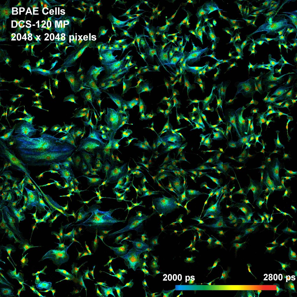
An example of a Mosaic-FLIM image is shown
in Fig. 2. The image was recorded by a DCS-120 MP (multiphoton) system in
combination with a bh SPC-160 TCSPC system [1]. The mosaic has 4 x 4
elements, each element has 512 x 512 pixels with 256 time channels. The
complete mosaic has thus 2048 x 2048 pixels, each pixel containing
256 time channels. The sample area covered by the mosaic is 0.8 mm x 0.8 mm.
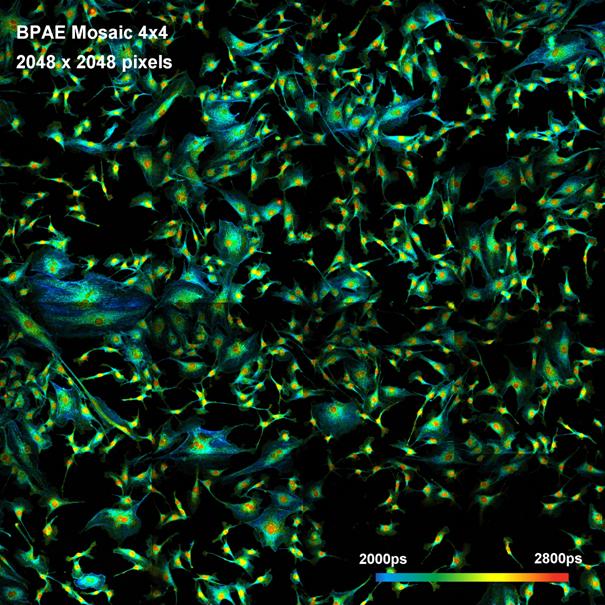
Fig. 2: Mosaic FLIM of a BPAE cell
sample. The mosaic has 4x4 elements, each element has 512x512 pixels, each
pixel has 256 time channels. DCS-120 MP (multiphoton) system. Data analysis by bh SPCImage. Use Adobe zoom function to see image
at higher resolution.
Integration in SPCM
Fig. 3 shows how the optical scanner
interacts with the motor stage. When Mosaic (Tile) Imaging is enabled the step
width of the motor stage automatically adjusts to the scan area (Zoom factor)
selected in the DCS-120 scanner panel. When the measurement is started the SPC
system records a mosaic of FLIM images the elements of which have the same x
and y size as the step width of the motor stage. The data of the individual
elements of the mosaic (or tiles) can be accumulated over a selectable number
of frames (20 in Fig. 3). The number of frames per mosaic element can be
selected both in the motor stage panel and in the scanner panel.
Fig. 3: Interaction of the motor stage
with the DCS-120 scanner
The size of the DCS scan area differs for
different optical systems and for different microscope lenses. To guarantee
that the individual tiles fit together seamlessly the step width of the motor
stage can be calibrated. The calibration panel is shown in Fig. 4. The
calibration table contains the size, X and Y, of the field of view (scan area)
of the optical scanner for Zoom = 1. The calibration factors can (but need not)
be made different in x and y to account for possible tolerances in the drivers
of the galvanometer mirrors. Up to six calibration values can be defined for
different microscope configurations or objective lenses.
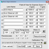
Fig. 4: Calibration of the motor stage
Advantages
Large-area FLIM images are normally
recorded by simply using low-magnification microscope lenses. However, such
lenses have low NA (numerical aperture). Low NA results in low light collection
efficiency, low excitation efficiency for multiphoton excitation, and poor
optical resolution. With mosaic FLIM, large image areas can be covered with
high-NA objective lenses. The result is high efficiency, both for excitation
and collection, and high spatial resolution. Since the entire mosaic is
recorded into a single, large FLIM photon distribution, standard SPCImage FLIM
data analysis [1] can be applied to the data.
References
1. W. Becker, The bh TCSPC handbook. 7th edition. Becker & Hickl
GmbH (2017), www.becker-hickl.com
2. W. Becker, Introduction to Multi-Dimensional TCSPC.
In W. Becker (ed.) Advanced time-correlated single photon counting
applications. Springer, Berlin, Heidelberg, New York (2015)
3. Becker & Hickl GmbH, DCS-120 Confocal Scanning FLIM Systems,
user handbook. Available on www.becker-hickl.com
Contact:
Becker & Hickl
GmbH
Berlin, Germany
info@becker-hickl.com