New SPCImage Version Combines Time-Domain Analysis with Phasor Plot

Wolfgang Becker, Axel Bergmann, Becker & Hickl GmbH, Berlin, Germany

Abstract: Version 6.0 SPCImage FLIM analysis software combines time-domain multi-exponential decay analysis with the phasor plot. In the phasor plot, the decay data in the individual pixels are expressed as phase and amplitude values in a polar diagram. Independently of their location in the image, pixels with similar decay signature form clusters in the phasor plot. Different phasor clusters can be selected, and the corresponding pixels back-annotated in the time-domain FLIM images. The decay functions of the pixels within the selected phasor range can be combined into a single decay curve of high photon number. This curve can be analysed at high accuracy, revealing decay components that are not visible by normal pixel-by pixel analysis.

The Phasor Plot

TCSPC-FLIM data can be analysed both in the time-domain and in the frequency domain. Time-domain analysis fits the decay data in the individual pixels with a single or multi-exponential decay model, or calculates lifetimes via the first moment of the decay functions [1]. Frequency-domain analysis transforms the decay data into the frequency-domain, and expresses the decay data as amplitude and phase values at subsequent harmonics of the repetition frequency. As it turns out, a good representation of the decay signature is obtained already if only the phase and the amplitude at the fundamental repetition frequency is used. Such data describe the fluorescence decay in each pixel by just two numbers - the phase and the amplitude of the first Fourier component.

Phase / amplitude data can be displayed and analysed elegantly by the ‘Phasor’ approach developed by the group of Enrico Gratton. For each pixel, a pointer (the ‘phasor’) is defined and displayed in a polar plot. The phase is used as the angle of the pointer, the modulation degree as the amplitude [2, 3]. This ‘phasor plot’ has several remarkable features:

- The phasors of pixels with single-exponential decay profiles are located a semicircle. The location on the semicircle depends on the fluorescence lifetime

- Phasors of combinations of several decay components are linear combinations of the phasors of the components

- Phasors of pixels with multi-exponential decay profiles, i.e. sums of several decay components, end inside the semicircle

- Pixels with similar amplitude-phase values form clusters in the phasor plot. Pixels with similar decay signature can thus be identified in the phasor plot, and combined for further analysis or back-annotated in the image

Phasor analysis does not explicitly aim on determining fluorescence lifetimes or decay components for the pixels. Instead, it uses the phase and the modulation degree directly to separate or identify fluorophores or fluorophore fractions, and determine concentration ratios of different fluorophore fractions. The principle of the phasor approach is shown in Fig. 1.

Fig. 1: Relations between decay functions in the time domain (left) and phasors in the frequency domain (right)

Implementation in SPCImage

Fig. 2 shows the main panel of the SPCImage data analysis [1]. Data have been loaded, and analysed with a double-exponential decay model. The panel shows an intensity image, a lifetime image of the amplitude-weighted lifetime, a lifetime histogram over the pixels, the decay curve at a selected position, and the corresponding decay parameters. The images in Fig. 2 show cells expressing two fluorescent proteins. In two of the cells (the green and orange one) the proteins are interacting, and FRET occurs. The result is a double-exponential decay with a slow and a fast component from the non-interacting and interacting donor, and, consequently, decrease in the fluorescence lifetime [1]. The lifetime differences are clearly seen in the lifetime image. The lifetime histogram shows three distinct peaks for the different cells.

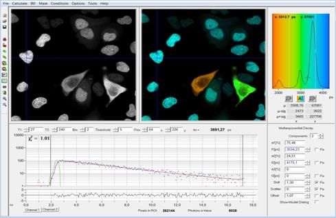
Fig. 2: SPCImage main panel. Intensity image, lifetime image, lifetime histogram, decay curve at selected position, and decay parameters at selected position. Recorded by bh Simple-Tau 152 FLIM system with Zeiss LSM 880.

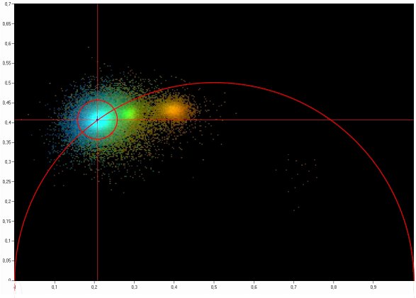
A click into ‘Tools’, ‘Phasor Plot’ opens the phasor plot panel. The relations between the lifetime image and the phasor plot are shown in Fig. 3. Every pixel in the FLIM image (left) is represented by a dot in the phasor plot (right). Pixels inside areas with different decay profiles in the lifetime image are thus represented as different clusters of phasors in the phasor plot. To make the correspondence between the image and the phasor plot clearly visible SPCImage can assign the colours of the FLIM image to the dots in the phasor plot. This function is activated by activating the ‘Combine with FLIM analysis’ option in the phasor plot. Cells of different lifetimes therefore form separate clusters of phasors marked with different colours in the phasor plot, see Fig. 3, right.

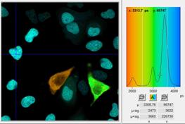
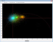
Fig. 3: Left: Lifetime image and lifetime histogram. Right: Phasor plot. The clusters in the phasor plot represent pixels of different lifetime in the lifetime image. Recorded by bh Simple-Tau 152 FLIM system with Zeiss LSM 880.

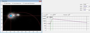
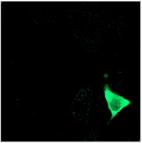
A cluster of interest in the phasor plot can be selected by a cursor. By activating ‘select cluster’ only pixel areas with phasors inside the selected cluster area are displayed in the lifetime images, see Fig. 4, right. ‘Sum up decay curves’ in this situation combines the decay data of all pixels inside the selected cluster area in a single decay curve, see Fig. 4, middle. The result is a curve with an extremely high photon number, as it is normally obtained only in a cuvette measurement. This curve can be analysed at very high accuracy. In the case shown in Fig. 4 the combined data show clearly that the blue cells have no interaction of the donor with an acceptor. The decay function is a single exponential from the donor, with the cluster on the semicircle in the phasor plot and two identical lifetime components in the time-domain fit. The green cell has weak FRET, with an interacting donor fraction of 1.95 ns lifetime. The yellow cell has strong FRET, with an interacting donor fraction of 708 ps.

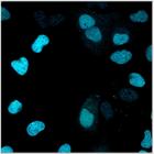
                                                           (Figure continued page 4)

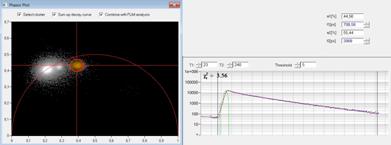
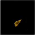
Fig. 4: Left: Selecting a cluster of phasors in the phasor plot. Middle: Combination of the decay data of the corresponding pixels in a single decay curve. Right: Display of the pixels corresponding to the selected cluster in the phasor plot. Top to Bottom: Selection of different phasor clusters selects cells with different decay signature.

Discussion

The combination of the phasor plot with time domain fluorescence decay analysis identifies pixels of similar decay signature in the frequency domain and back-annotates the corresponding image areas in the time-domain FLIM images. This provides an intrinsic image segmentation function. Separate images of different cells, different anatomic features with characteristic decay signature or images for selected fluorophores or fluorophore fractions can be obtained. The decay data of the pixels within these areas can be combined in a single curve with substantially increased photon number. This curve can be analysed at an accuracy comparable to that of single-point decay measurements in cuvettes. Low-amplitude decay components or decay components with almost similar lifetimes can thus be identified in the data. It should be noted that pixels of similar signature can also be selected in multi-parameter histograms in the time domain. These histograms either use several independent parameters of multi-exponential decay functions [1] or fluorescence decay times and intensity ratios in different wavelength intervals [4]. Also these approaches deliver clusters of pixels with similar decay signature. The advantage of the phasor plot is that the clusters are usually more clearly defined than in decay parameter histograms, or do not depend on amplitude ratios which may vary with filters, detectors, and absorption in the sample. It should be noted, however, that all the cluster approaches are not always unambiguous. Similar phasors or similar intensity ratios are not necessarily meaning that the decay profiles of the corresponding pixels are similar. It is an advantage of the method presented here that the combined decay profiles can be analysed at high precision, and the source of unexpected decay components be identified.

Acknowledgements

The data used in this application note were recorded on the EMBO Workshop on Biomolecular Interaction Analysis 2016: From Molecules to Cells, in Porto, Portugal, 2019. We thank Kees Jalink of NKI Amsterdam and Ana Seixas and Maria Azevedo, IBMC Porto for donating the cell material and preparing the samples. Moreover, we thank Uros Krzic of Zeiss for donating an LSM 880 to the FLIM experiments, and Valeria Caiolfa and Moreno Zamai for organising the tutorial session.

References

1.            W. Becker, The bh TCSPC Handbook, 6th edition. Becker & Hickl GmbH (2015). Available on www.becker-hickl.com, printed copies available from bh

2.            Digman, M.A., Caiolfa, V R., Zamai, M. & Gratton, E.  The phasor approach to fluorescence lifetime imaging analysis. Biophysical J. 94, L14-L16 (2008)

3.            M.A. Digman, E. Gratton, The phasor approach to fluorescence lifetime imaging: Exploiting phasor linear properties. In: L.Marcu, P.W.M. French, D.S. Elson, Fluorescence lifetime spectroscopy and imaging. CRC Press, Taylor & Francis Group, Boca Raton (2015)

4.            S. Weidkamp-Peters, S. Felekyan, A. Bleckmann, R. Simon, W. Becker, R. Kühnemuth, C.A.M. Seidel. Multiparameter fluorescence image spectroscopy to study molecular interactions. Photochem. Photobiol. Sci. 8, 470-480 (2009)