Live bacteria are often difficult to image in their natural environment because they are extremely mobile. To obtain reasonable image quality extremely short image acquisition time has to be used which, however, leads to pixel photon numbers insufficient for accurate lifetime analysis. Higher excitation power does not solve the problem because it impairs the viability of the bacteria or even causes severe photodamage. We therefore developed a FLIM technique that records a sequence of fast single-frame images, identifies the bacteria in these images by phasor analysis, and combines the photons of the corresponding pixels in a single decay curve of high photon number. This curve is processed by multi-exponential decay analysis in the time-domain, yielding precision multi-exponential decay parameters of the bacteria.

Keywords: FLIM, Label-Free, NADH, Metabolic Imaging, Moving Bacteria, Phasor Plot

Related Applications

Related Application Notes

Download PDF

Label-Free Multiphoton FLIM of Moving Bacteria

Wolfgang Becker, Axel Bergmann, Julius Heitz, Becker & Hickl GmbH, Berlin, Germany

Abstract: Live bacteria are often difficult to image in their natural environment because they are extremely mobile. To obtain reasonable image quality extremely short image acquisition time has to be used which, however, leads to pixel photon numbers insufficient for accurate lifetime analysis. Higher excitation power does not solve the problem because it impairs the viability of the bacteria or even causes severe photodamage. We therefore developed a technique that records a sequence of fast single-frame images, identifies the bacteria in these images by phasor analysis, and combines the photons of the corresponding pixels in a single decay curve of high photon number. This curve is processed by multi-exponential decay analysis in the time-domain, yielding precision multi-exponential decay parameters of the bacteria.

Autofluorescence FLIM

Biological material contains a number of fluorescent compounds which can be used for fluorescence imaging. The most interesting one is NAD(P)H (nicotinamide adenine (pyridine) dinucleotide). NAD(P)H is not only involved in the metabolism of the cell, its fluorescence also depends on the type of the metabolism. The effect is difficult to see by spectral imaging, but can reliably be resolved by FLIM. It then reveals itself by different amounts of fast and slow decaying fluorescence [1, 13, 18]. NAD(P)H FLIM - or NAD(P)H FLIM combined with FAD FLIM - is therefore also called 'Metabolic FLIM' [5, 6]. It is being used in a large number of life-science applications [11, 12, 15, 17, 19]. Please see [1] for an overview on the literature. A FLIM image of Streptococcus Salivarius bacteria is shown in Fig. 1. The decay curves show the typical multi-exponential behaviour of NAD(P)H. The fast component has a decay time of 361 ps and comes from free NAD(P)H. The slow fluorescence is split in two components of 1.956 ns and 5.395 ns and comes from bound NADPH and bound NADH [10].

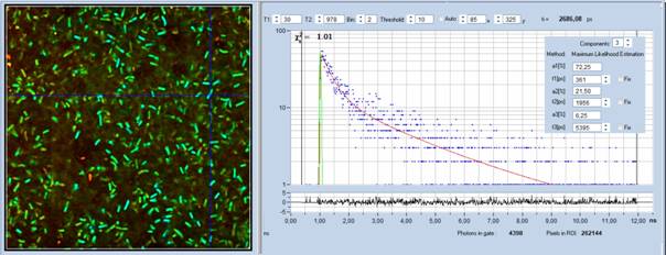
Fig. 1: NADH FLIM image of Streptococcus Salivarius. bh DCS-120 MP FLIM system, excitation at 785 nm, detection from 440 nm to 480 nm. Decay curve and decay parameters at cursor position shown in the right.

NAD(P)H imaging requires an excitation wavelength of 340 to 380 nm. Wavelengths this short are difficult to handle in a microscope. The transmission of the optics is far from ideal, and there are large aberrations which impair the spatial resolution. NAD(P)H FLIM is therefore usually performed by two photon excitation. Moreover, metabolic FLIM has to be performed on live cells and tissues with intact metabolism. The applicable excitation power is therefore very limited, and the fluorescence intensities are low. In principle, this is no problem for bh's TCSPC FLIM [1, 2]. The timing stability of the technique is so high that technically the acquisition time is virtually unlimited. A sufficient number of photons can therefore always be acquired by simply extending the acquisition time. Typical acquisition times are in the range from 10 seconds for medium lifetime accuracy and low pixel numbers to several minutes for precision measurements. This is not very long but can cause a problem if the objects of interest in the sample are moving.

The Problem

Motion in live samples is the nightmare of any FLIM user. To acquire enough photons for precision decay analysis a large number of frames have to be accumulated. This is no problem as long as the objects in the sample stay in place for the entire acquisition time. However, if the objects under investigation are moving, as bacteria do, the image is smeared out, and the decay data of the bacteria are mixed with signals from the substrate. The first idea in these cases is usual to pull up the excitation power and thus increase the photon flux. A given accuracy of the decay data would then be reached in a shorter acquisition time. Unfortunately, the options of this approach are very limited. High excitation power quickly causes invasive effects or even catastrophic damage in the sample, rendering the FLIM results useless. This is especially the case in autofluorescence experiments where the emission from the cells is weak.

An example is shown in Fig. 2. The images show live Escherichia coli bacteria on the substrate they were cultured on. The data were recorded with a bh DCS-120 MP Fibre-Laser system at 785 nm excitation wavelength. The bacteria are extremely mobile. Recorded at an acquisition time of 1.5 seconds the bacteria are still marginally visible (left image). However, the photon numbers in the pixels are not sufficient for multi-exponential decay analysis. Another problem that shows up in Fig. 2 is background fluorescence from the substrate. For immobile object it is suppressed by the depth resolution of the two-photon excitation process. For objects that move during the acquisition, however, fluorescence of the background is mixed into the fluorescence of the objects.

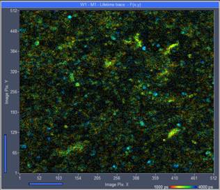
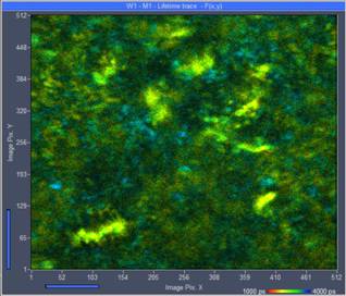
Fig. 2: Left: Escherichia coli bacteria culture, single scan of 1.5 second duration. The bacteria are marginally visible, but there are not enough photons for accurate lifetime analysis. Right: Same sample, acquisition time 24 s. There are enough photons per pixel but motion has rendered the bacteria invisible.

With the acquisition time increased to 24 seconds (Fig. 2, right) the motion has totally smeared out the image detail. Only immobile bacteria are still visible. These bacteria have unusually long lifetimes. They are probably not the viable ones and are thus not interesting for further investigation.

As mentioned above, it is usually attempted to solve the problem by higher excitation power. Higher excitation power yields, of course, a higher rate of fluorescence photons and thus a better image in a shorter period of time. But this comes at a price. Fig. 3 shows a recording with 2.5 times increased excitation power. This leads to a 6.52 fold increase in photon rate. No doubt bacteria are better visible than in Fig. 2, but a large number of spots with extremely short lifetimes (red in the image) have appeared. These are burn marks which indicate that severe photodamage has occurred. Of course, there are still bacteria which appear to be intact. However, with severe photodamage present nearby, the decay data and, especially, the metabolic information derived from them cannot be trusted.

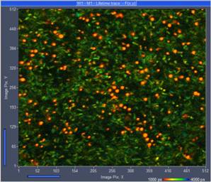
Fig. 3: FLIM recording at 2.5 x increased laser power. The red spots of ultra-short lifetime indicate sample damage. Online-lifetime display of SPCM, red to blue = 1 ns to 4 ns.

The problems shown in Fig. 2 and Fig. 3 have led to an avalanche of demands for faster FLIM techniques. These solutions are designed to work at high photon flux, but at the expense of photon efficiency [4, 14]. Of course, the approach was not successful, leading to the conclusion that FLIM is not a suitable technique for molecular imaging. Of course, this is wrong. Where is the mistake?

The limitation of acquisition speed is in the ability of the sample to deliver high photon rates, not in the counting capability of the FLIM technique. Increasing the counting capability at the expense of photon efficiency makes the situation worse. More photons are needed to reach a given accuracy level, with the result that damage effects become even more severe. Unless the samples are extremely bright and stable (which is not the case in molecular imaging applications [1]) TCSPC FLIM is and remains to be the fastest technique because it needs less photons than 'fast' FLIM techniques.

The Solution

Image Segmentation by Phasor Plot

So, how can the problem of motion in the samples be solved? Obviously, not with a faster FLIM technique. A possible way to obtain decay information from the moving bacteria would be to record a single, fast scan, identify the bacteria in the image, and sum up the decay data of all pixels which are located inside the bacteria. The resulting curve will contain a significantly higher number of photons than a single pixel.

How can the bacteria be identified in the image of a single scan? A simple (and readily available) way is the phasor plot of bh's SPCImage NG FLIM data analysis, please see [1, 7, 9]. The phasor plot reacts very sensitively to differences in the signature of the decay data in the pixels. Pixels of similar decay signature are located close to each other in the phasor plot. Even if the photon number is too low for pixel-by-pixel analysis the phasor range of the bacteria can be indentified. The phasor range of interest is then marked by the operator, and the corresponding pixel are back-annotated in the image. The decay data in these pixels are summed up, and the resulting curve is analysed by the normal time-domain fit routine.

The procedure is illustrated in Fig. 4. A single-frame image is shown on the left. As expected, standard decay analysis does not deliver precision decay data of the bacteria, see decay data lower right. Nevertheless, the maximum-likelihood fit of SPCImage NG delivers an approximate lifetime (shown by colour) in the image. The phasor plot (upper right) shows a cloud of phasor values for the individual pixels of the scan. Selecting a range of phasors of the same colour as the bacteria (compare FLIM image on the left) selects the pixels inside the bacteria.

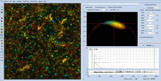
Fig. 4: Single-frame data loaded into SPCImage NG. Left: Lifetime image, approximate lifetime. Upper right: Phasor plot. Lower right: decay curve at cursor position.

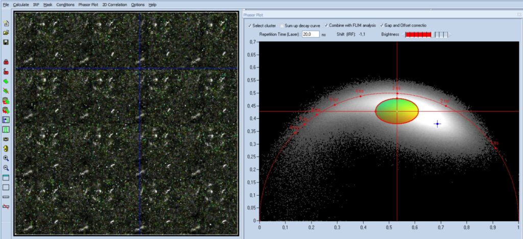
When an appropriate phasor range has been selected, the 'Select Cluster' function is activated, see Fig. 5, upper left of phasor plot. This suppresses analysis of pixels outside the selected phasor range. The result can be seen in the lifetime image. It indeed selects the bacteria, showing that the phasor range was estimated correctly. Now activate 'Sum Up Decay Curve'. This combines the decay data of all pixels of the selected phasor range into a single decay curve. The resulting curve has a large number of photons (see lower right) and can be analysed at high accuracy. In Fig. 5 a fit with a double-exponential model was used. It delivers the average decay parameters of the bacteria, see upper right. The component amplitudes, a1 and a2, and the component lifetimes, t1 and t2, are shown in the upper right. All parameters are well in the range expected for NAD(P)H.

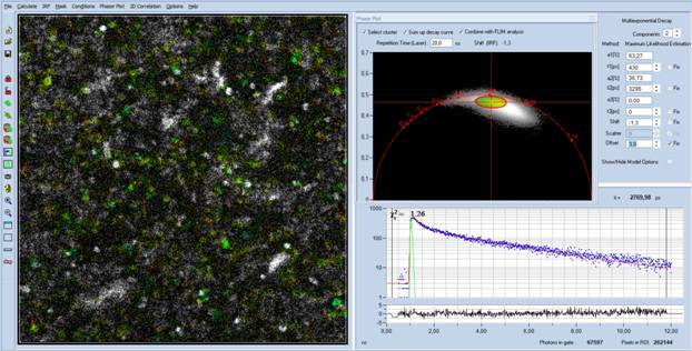
Fig. 5: Data from Fig. 4, 'Select Cluster' and 'Sum Up Decay Curve' active. The decay data of the selected phasor range are combined into a single decay curve, representing the average decay curve of the bacteria. The decay parameters (upper right) are as expected for NAD(P)H.

Mosaic FLIM with Image Segmentation by Phasor Plot

The method described above works well if there is a sufficient number of objects in the image and if the expectations to the decay accuracy are moderate. If this is not the case a more powerful procedure can be used. The idea behind it is: If image segmentation in a single scan is effective to derive a high accuracy decay curve then segmentation in several scans will be even more effective.

We have shown above that a single fast scan delivers an reasonably sharp image in which moving objects can be identified. A second fast scan will deliver a sharp image as well. However, the bacteria will have moved to different places, some of them may have moved out of the focal plane, and other may have moved in. In other words, every scan shows a different image. If the objects are identified in all these single-scan images and the decay data of the corresponding pixel be summed up the increase in photon number will be even more dramatic than in a single scan. Moreover, in contrast to the approach described above the Mosaic approach works also for a single object in the field of view which is either moving or changing its shape [8].

The procedure is illustrated in Fig. 6 to Fig. 8. A mosaic of FLIM images is recorded by the Mosaic recording function of SPCM data acquisition software [1]. The result is shown in Fig. 6. Please note that it is not required to move the sample from one mosaic element to the other - the images of subsequent scans are different anyway. The entire mosaic is loaded into SPCImage NG, a preliminary FLIM analysis is performed, and the phasor plot is opened, see Fig. 7. The phasor range formed by the bacteria is selected and the photons of the corresponding pixels are summed up, see Fig. 8. The result is a decay curve that has an accuracy previously known only for cuvette-based measurement. A fit of the resulting decay curve with a triple-exponential model delivers the decay parameters of the bacteria, see Fig. 8, upper right. The fit even splits the slow fluorescence into two decay components, known to come from bound NADH and bound NADPH [10].

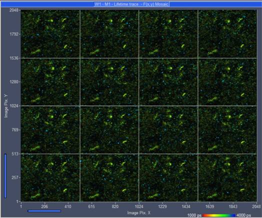
Fig. 6: 4x4 Mosaic of single scans, recorded by Mosaic Imaging function of SPCM data acquisition software. Displayed by online-lifetime function of SPCM. The data structure of mosaic resembles that of a single, large FLIM image.

Fig. 7: 4x4 mosaic, loaded into SPCImage NG. Phasor plot enabled, phasor range of bacteria selected, selected pixels back-annotated in the FLIM image.

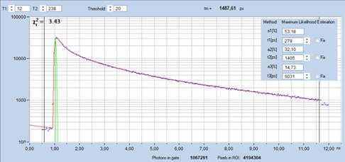
Fig. 8: Decay curve obtained by summing up decay data of pixels selected by phasor plot. Fit with SPCImage NG, triple-exponential 'incomplete-decay' model. Total number of photons 1,067,291, Decay parameters shown upper right.

Summary

Molecular imaging by FLIM often faces the problem that the objects of interest in the sample are moving. Reasonable images are then only achieved by imaging with short acquisition time. However, molecular imaging not only has to be performed on live samples but is also connected to low fluorophore concentrations and fluorophores of low quantum yield. The number of photons obtained from the sample within a short period of time is then not sufficient for accurate multi-exponential decay analysis. A solution of the problem lies in a combination of time-domain analysis and phasor analysis. Pixels within the objects are identified via the phasor plot and the decay data of these pixels are combined into a single curve. The combined data contain enough photons for decay analysis. An even more dramatic improvement is obtained by combining this procedure with the Mosaic Imaging function of the bh FLIM systems. The photon number obtained this way is comparable with the photon number in cuvette-based fluorescence-lifetime measurements. Consequently, precision analysis of the decay curve is possible. We show that the data quality obtained this way is so high that precision triple-exponential decay analysis of NAD(P)H is possible.