We describe a TCSPC FLIM system that uses 8 parallel TCSPC channels to record FLIM data at a peak count rate on the order of 50⋅10⁶ s^-1. By using a polychromator for spectral dispersion and a multi-channel PMT for detection we obtain multi-spectral FLIM data at acquisition times on the order of one second. We demonstrate the system for recording transient lifetime effects in the chloroplasts in live plants.

Related Application Notes

Multiphoton Multiwavelength NDD FLIM with Zeiss LSM 710 NLO

Download PDF

An 8-Channel Parallel Multispectral TCSPC FLIM System

Abstract. We describe a TCSPC FLIM system that uses 8 parallel TCSPC channels to record FLIM data at a peak count rate on the order of 50×10⁶ s^‑1. By using a polychromator for spectral dispersion and a multi-channel PMT for detection we obtain multi-spectral FLIM data at acquisition times on the order of one second. We demonstrate the system for recording transient lifetime effects in the chloroplasts in live plants.

Count Rates in TCSPC FLIM Experiments

TCSPC FLIM [3, 6] delivers single- and multi-wavelength fluorescence lifetime images at an accuracy essentially limited by the photon statistics [1, 11], and a time resolution limited by the transit-time-spread of the detector [4, 5, 12]. This is a clear advantage in the typical FLIM applications, such as FRET measurements, investigation of membrane proteins, or autofluorescence imaging. All these applications have in common that the fluorophore concentration is low. Moreover, the excitation power has to be kept low to avoid cell damage and lifetime changes by photobleaching. The count rates available from the samples are therefore on the order of only 10⁴ s^‑1 to a few 10⁵ s^‑1. This is one to two orders of magnitude lower than the counting capability of a single TCSPC FLIM device [5]. Consequently, the acquisition time required to achieve a given lifetime accuracy is exclusively given by the photostability of the sample, not by the counting capability of the TCSPC module. Technical efforts to increase the counting capability of the TCSPC FLIM electronics therefore do not result in shorter acquisition times in these applications.

There are, however, certain classes of FLIM experiments that can be run at very high count rate. One of these is imaging of chlorophyll in plant tissue. Chlorophyll is highly photostable and emits strong fluorescence around 700 nm. The fluorescence lifetime of chlorophyll in live plants changes with the time of exposure [9]. Recording these changes requires fast FLIM [10]. Another potential application is, surprisingly, autofluorescence. Autofluorescence signals are usually weak, but exceptions do exist. Fig. 1 shows autofluorescence FLIM images of live yeast cells. The bright cells (probably apoptotic ones) are about 50 times brighter than the dim ones (visible only in Fig. 1, right).

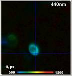
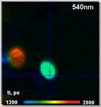
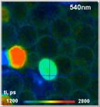
Fig. 1: FLIM images of yeast cells. Left: Intensity scale 0 to 3000 counts per pixel. Right: Intensity scale 0 to 300 counts per pixel. The bright cells are about 50 times brighter than the dim ones. Becker & Hickl DCS-120 confocal scanning FLIM system, excitation at 407 nm.

Recording lifetimes for both types of cells in the same image requires the count rate of the bright cells to be kept below about 4 MHz. The count rate in the dim cells is then less than 100 kHz. The high contrast thus results in an unnecessarily long acquisition time.

The Way to Higher Counting Capability

The count rate of TCSPC FLIM is limited by counting loss due to the dead time of the TCSPC electronics, by pile-up effects, and saturation in the detector [4, 5, 10]. Counting loss could, in principle, be reduced by decreasing the dead time of the electronics. Pile-up-effects could be reduced by recording more than one photon per signal period. Unfortunately, both approaches have detrimental effects on the accuracy of the FLIM data. Reducing the dead time increases the background caused by the afterpulsing of the detector [4]. Recording several photons per laser period leads to an overlap of subsequent single-photon pulses and thus causes count-rate-dependent distortions of the decay curves [10]. In any case, detector nonlinearity and detector overload preclude the use of a single detector at count rates much higher than 10⁷ s^‑1.

A better way to increase the counting capability of TCSPC FLIM is therefore to use several parallel TCSPC channels. Standard FLIM systems for the bh DCS-120 confocal scanner [7] or the Zeiss LSM 710 NLO [8] system therefore have two parallel TCSPC channels. Four-channel FLIM systems are available as well [5] and have been shown to record FLIM at an average count rate of 13 MHz [2].

8-Channel Parallel FLIM

To further increase the counting capability of TCSPC FLIM we built an eight-channel parallel FLIM system. The architecture of the system is described below. We use the Becker & Hickl DC‑120 confocal scanning FLIM system [7], see Fig. 2, left. An LOT MS 125 polychromator is attached to one confocal output of the DCS‑120 scanner. The polychromator is used without an input slit; the light focused into the slit plane by a lens.

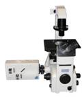
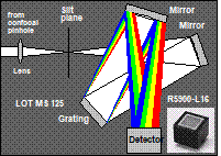
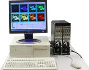
Fig. 2: Eight-channel FLIM system. Left: DCS‑120 scanner. Middle: Principle of spectral dispersion. Right: FLIM electronics.

The spectrum at the polychromator output is detected by a Hamamatsu R5900‑L16‑01 multichannel PMT. Only eight of the 16 channels of the R5900 are used; the remaining ones are terminated via 50 W into ground. Alternatively, connecting every two PMT channels in parallel is possible, but not recommended. The PMT channels have slightly different signal transit times. Connecting channels in parallel thus impairs the time resolution. Moreover, combining channels would also combine the dark counts and thus result in an unwanted increase of the thermal background.

The electronics of the 8-channel FLIM system is shown in Fig. 2, right. We use two Simple-Tau 154 bus extension boxes holding four bh SPC‑150 TCSPC modules each. The boxes are connected to a standard Pentium PC via bus extension cables. The PC also contains a DCC‑100 detector controller card [5] and the scan controller card of the DCS‑120 system [7].

Fig. 3 shows autofluorescence FLIM of a Drosophila eye. The excitation wavelength was 407 nm. The images were scanned at a resolution of 256 x 256 pixels and a rate of 500 ms per frame. The intensities were normalised on the brightest pixels.

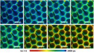
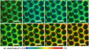
Fig. 3: Multi-wavelength FLIM of a Drosophila eye. Autofluorescence, excitation at 407 nm. Double-exponential decay model. Left: Amplitude weighted mean lifetime. Right: Relative amplitude of fast decay component.

The total count rate (summed over all TCSPC channels and averaged over the image) obtained from the Drosophila eye was about 4×10⁶ s^‑1. That means the rate in the brightest pixels was more than 10×10⁶ s^‑1. A single‑channel FLIM system would still deliver reasonable lifetimes under these conditions but inevitably develop visible intensity nonlinearity.

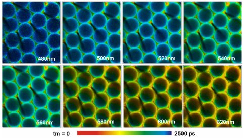
A time-series recording with the 8-channel system is shown in Fig. 4. A moss leaf was scanned with 407 nm excitation wavelength, and at a scan rate of 4 frames per second. The data format of the TCSPC data was 256 x 256 pixels x 256 time channels. The lifetime shown is an amplitude-weighted average of the two lifetime components of a double-exponential fit. The intensity scale of all images was normalised on the intensity of the brightest pixel.

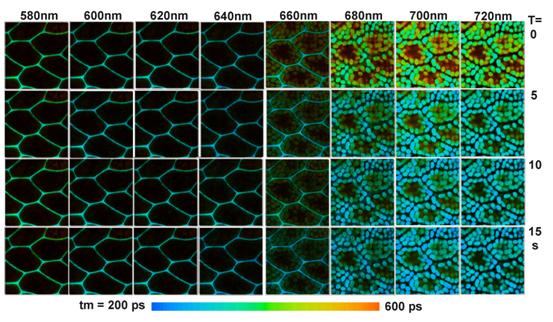
Fig. 4: Multi-wavelength time-series FLIM obtained from a moss leaf. Each image is 256 x 256 pixels, 256 time channels. Left to right: Wavelength, from 580 nm to 720 nm. Top to bottom: First four steps of the time series, acquisition time 5 seconds per step.

In the wavelength intervals from 580 nm to 640 nm the fluorescence comes from the cell membranes. At 660 nm fluorescence of the chloroplasts starts to show up. From 680 nm to 720 nm the images are totally dominated by chlorophyll fluorescence. The lifetime of the chloroplasts decreases over the time of exposure, due to induction of a non-photochemical quenching transient. The lifetime in the cell membranes remains constant.

The variation of the lifetime can be seen more clearly in Fig. 5. The figure shows lifetime images in the 700 nm interval for the first four steps of the time series. The lifetime scale has been stretched to 200 ps to 400 ps. Decay curves in a selected spot of the images are shown in the second row.

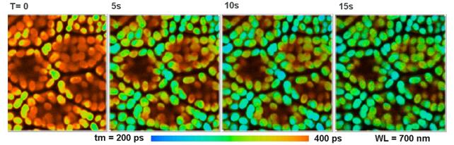
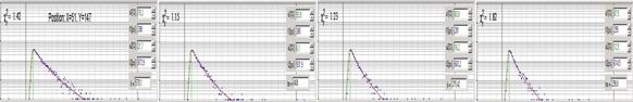
Fig. 5: First four steps of the time series, 700 nm interval. Upper row: Lifetime images. Lower row: Decay curve in pixel position X=51, Y=147.

Summary

The results presented show that an eight-channel parallel TCSPC FLIM system is feasible and operable. The advantage over a single-channel multispectral FLIM system [5, 6] is that the applicable count rate is 8 times higher. Moreover, possible saturation in a single spectral channel does not cause artefacts in other channels.

The parallel-channel architecture allows relatively large FLIM data formats to be used. However, large pixel and time channel numbers in combination with the eight channels result in large data file size. Every single recording step of the time-series shown in Fig. 4 produces 260 Mbytes of data. The rate at which a time series can be recorded is thus limited by the speed at which the computer can save the data. The rate scales with the image format; for images of 128 x 128 pixels x 256 time channels a speed of about 1.3 seconds per step is reached.

It should be noted that the 8-channel system is built from standard components of the bh modular FLIM systems. Moreover, the application of the system is not restricted to bh DCS-120 confocal scanning system. It can be used with any confocal or multiphoton laser scanning microscope that gives the user access to the fluorescence light via an optical port.