Combined Fluorescence and Phosphorescence Lifetime
Imaging (FLIM / PLIM) with the Zeiss LSM 710 NLO Microscopes
Wolfgang Becker, Stefan Smietana, Axel Bergmann,
Becker & HIckl GmbH, Berlin, Germany
The PLIM
technique described here is based on modulating the titanium-sapphire laser of
a multiphoton microscope by a signal synchronous with the pixel clock of the
scanner, and recording the fluorescence and phosphorescence signals by
multi-dimensional TCSPC [1]. Fluorescence is recorded during the on-phase of
the laser, phosphorescence during the off-phase. Laser modulation is achieved
by controlling the the AOM of the laser scanning microscope by a signal
generated in the TCSPC system. This document contains instructions of how to set
the parameters of the bh SPC‑150 or SPC‑830 FLIM systems for
combined fluorescence (FLIM) and phosphorescence lifetime imaging (PLIM). It
should be considered a supplement to the bh TCSPC Handbook [1] and the bh
Handbook of the FLIM systems for the Zeiss LSM 510 and 710 laser scanning
microscopes [2].
Principle and System Architecture
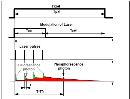
The general
principle of combined fluorescence and phosphorescence lifetime imaging is
shown in Fig. 1. A high-frequency-pulsed laser, in
this case the Ti:Sa laser of the LSM 710 NLO microscope, is used for
excitation. The laser is turned on for a short period of time, Ton, at the
beginning of each pixel [1, 3]. For the rest of the pixel time the laser is
turned off. Within the on-time the laser excites fluorescence, and builds up
phosphorescence. Within the rest of the pixel dwell time, Toff, pure
phosphorescence is obtained. Photon times are determined both with respect to
the laser pulses and with respect to the modulation pulse. The times from the
laser pulse, t, are used to build up the fluorescence decay. The
phosphorescence decay is built up from times from the modulation pulse, T-T0.
Fig. 1:
Principle of Microsecond FLIM
Because the
phosphorescence is built up over a large number of excitation pulses neither an
extremely high laser peak power is required, nor an extremely high fluorescence
peak intensity is generated. Saturation effects, both in the sample and in the
detector, are therefore avoided. Moiré effects in the image do not occur
because the laser-on/off modulation is synchronous with the pixel clock.
The system
architecture is shown in Fig. 2. The system uses a standard bh TCSPC FLIM
system that is connected to the LSM 710 NLO in the usual way [2]. To
generate the laser modulation signal a bh DDG‑210 programmable pulse
generator card is added to the system. The DDG-210 is triggered by the pixel
clock of the LSM 710. It delivers a laser modulation signal of programmable
width, which is fed back into the beam blanking system of the microscope, see Fig.
2, left. The feedback of the modulation signal requires a change in the
LSM 710 NLO laser controller. The changed controller is available via an
individual modification from Zeiss.
A second signal
is generated to indicate to the TCSPC module whether the laser is on or off. It
is used by the TCSPC module as a routing signal to send fluorescence and
phosphorescence photons into separate memory blocks [1]. The routing signal is
slightly delayed with respect to the modulation signal to account for the delay
in the opto-acoustic modulator (AOM) of the microscope, see Fig. 2, right.
Fig. 2: On-off modulation of LSM 710 laser. The pixel clock of the
LSM 710 triggers the generation of a laser-on pulse in the DDG-210 pulse
generator module. The laser-on pulse controls the beam blanking in the LSM 710.
The AOM of the LSM 710 responds to the beam blanking with a delay of a few
100 ns. A routing signal to the SPC-150 TCSPC module indicates when the
laser is on. Connection diagram shown left, pulse diagram right.
SPC System Parameter Setup
Combined FLIM / PLIM operation is obtained
without any hardware changes in the TCSPC module. It only requires appropriate
system parameter setup.
To set the parameters for FLIM / PLIM, open
the System Parameters panel of the SPCM software [1]. Click into the
Operation Mode field. Operation mode must be FIFO Imaging, see Fig. 3.
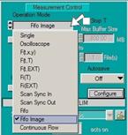
Fig. 3:
Operation mode
Open the Configure panel, see Fig. 4.
Enable both Picosecond FLIM and MCS (multichannel scaler) FLIM. Select the source
of the PLIM timing reference input. Timing reference for PLIM is the pixel
clock, which is identical with Marker 0. Select the number of time channels.
Recommended setting is 256. Select the desired time per point, or PLIM time
channel width. Time channel width is a multiple of the macro time clock (25 ns)
of the SPC module. The total time range of PLIM is the product of No. of
points and Time per point.
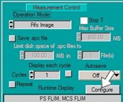
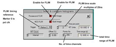
Fig. 4:
Defining MCS imaging, and MSC timing parameters
In the Page Control section of the system
parameters, set Routing Channels X = 2. One channel is for fluorescence, the
other for phosphorescence. Image pixels is the size of the FLIM image. The
typical value is 256 x 256. Larger and smaller images can be selected, see [1]
or [2]. Please note that the correct binning factors must be used in the scan
control parameters, see Fig. 6.
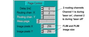
Fig.
5: Defining routing channels and FLIM / PLIM image size
To access the scan parameters, open More
Parameters in the system parameters panel. Define the scan parameters. Typical
settings for the Zeiss microscopes are shown in Fig. 6. The Line Divider and
Pixel Clock Divider values define the binning factor of the LSM scan into the
FLIM image. For the standard LSM scan of 512x512 and a FLIM image of 256x256
the binning factors must be 2. Please see [1] or [2] for details.
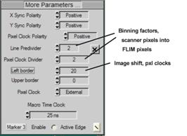
Fig. 6:
Defining scan parameters and binning from LSM scan into FLIM / PLIM images
Display setup
Window Intervals
Open the Window Intervals panel. Set the
parameters are shown below. The Routing X windows define three data channels.
Window 1 contains the photons during the Laser On time; window 2 contains the
photons during the Laser Off time. Window three contains all photons. Thus,
an image displayed for Window 1 shows the essentially fluorescence, an image
displayed for Window 2 shows phosphorescence. An image displayed for
window 3 contains both fluorescence and phosphorescence.
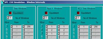

Fig. 7:
Defining routing window intervals
3D Trace Parameters
Open the 3D Trace parameter panel. Set the
parameters as shown below. The panel defines three images, one for Routing
window 1 (fluorescence, recorded by ps FLIM), one for Routing Window 2
(phosphorescence, recorded by MCS imaging), and one for the total luminescence
(Routing Window 3, recorded also by MCS imaging). The image for the total
luminescence has been turned off. To activate it click on the Window active
button.
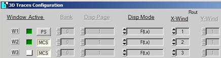
Fig.
8: Definition of display windows
Display parameters
The display parameter setup is the same as
for standard FLIM measurements [1, 2]. There are separate display parameters
for the FLIM and the PLIM window. The figure below shows a display for the PLIM
window. Note that you can change the Routing X Window in the display
parameters. With window intervals as shown above in Fig. 7 Routing X Window 1
is for the laser-on time, Routing X Window 2 is for the laser-off time, and Routing
X Window 3 is for the entire pixel time.
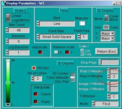
Fig.
9: Display parameters
Saving the setup data
Please dont forget to save the setup data.
Select the Save panel and follow the instructions given in [1] or [2]. For
frequently used setups we recommend to define an entry in the Predefined
Setup panel. Please see [1] for details.
DDG Setup
Start the control software of the DDG-210
pulse generator card. The general settings are shown in the panel below.
Repeat Sequence, Endless and Trigger on Positive Edge must be set.
Channel polarity is +. If the cables are connected as suggested in the system
cable plan the output of channel 1 controls the routing, the output of channel
2 the laser. You can use any other pair of outputs if you define the pulse
parameters of the channels accordingly.
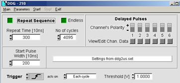
Fig.
10: DDG software panel
After starting the DDG software the DDG
automatically comes up with settings as they were used in the previous session.
If you want to run a PLIM experiment with the same excitation parameters as in
the session before there is no need to change anything. All you have to do is
to click the start button to start the DDG operation. See figure below.
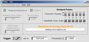
Fig.
11: DDG software panel, DDG is running
To change the Laser-On duration, click on
the View/Edit buttons of channel 1 and channel 2. Fig. 12 shows examples for a
laser-on duration of 2 us (left) and 8 us (right). The numbers shown are
the start times and the widths of the pulses in 10 ns units. Note that the
routing signal is shifted by 800 ns with respect to the laser-on pulse.
This compensates for the delay of the AOM (acousto-optical modulator) of the
microscope, which is about 800 ns. Please see also Fig. 2.
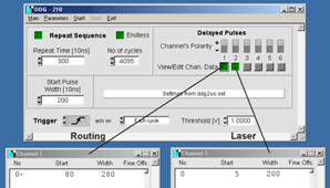
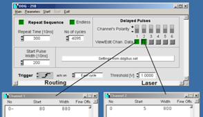
Fig. 12: DDG,
defining the laser modulation time parameters for PLIM
Note that you need a pixel time of the LSM
that is at least two times longer than the Laser On interval defined in the
DDG.
Running the measurement
Starting the measurement
The measurement is started as shown below.
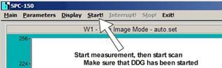
Fig.
13: Starting the measurement
Important:
When the measurement is started the SPC hardware waits for the beginning of a
new scan frame until it starts recording. The frame times used for PLIM can be
up to a minute or more. If the scan is already running when the measurement is
started it can take a long time until the recording begins. We therefore
recommend to start the measurement first, and then the scan in the LSM. The LSM
scan starts with a frame clock, thus the recording starts with the start of the
scan. Make sure that the DDG is running when you start the measurement.
Interpretation of count rates
The count rates present important
information on whether the intensity is within reasonable limits and the
recording process is running as expected.
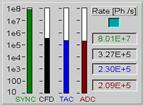

Fig.
14: Count rates
When running PLIM experiments, bear in mind
that the count rates are determined over intervals of one second. Different
than for FLIM, the excitation laser is only active for a short period of time
at the beginning of each pixel. The sample may emit strong fluorescence during
the laser-on time, but only weak phosphorescence for the rest of the pixel
time. The fluorescence count rate (during the laser-on time) can therefore be
considerably higher than the count rate displayed. If it exceeds a rate of
about 5 MHz the fluorescence decay profiles may be distorted by counting loss
and pile-up effects [1]. If the fluorescence count rates are so high that the
detector overloads also the phosphorescence decay data may be impaired.
Stopping
the measurement
There are two ways to stop a measurement:
The measurement can be stopped after a defined acquisition time or by an
operator command.
Stopping after a defined time is used when
the intensities (photon numbers) in the data of several measurements must
remain comparable. To stop after a given time, define the desired Collection
Time and activate the Stop T button. Stop T and Collection Time can be
defined either in the main panel or in the system parameters, see Fig. 15.
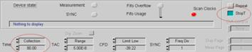
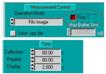
Fig. 15: Setup
for stopping the measurement after Collection time
In most cases, however, intensity information
in FLIM / PLIM data is not relevant. It is then more convenient to turn off
Stop T and stop the measurement manually when a reasonable signal-to-noise
ration is reached. See figure Fig. 16.
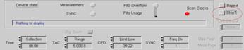
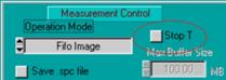
Fig. 16:
Setup for stopping the measurement by the operator
PLIM Data Analysis
Sending data to SPCImage
There are two ways to load data into the SPCImage
data analysis: An sdt file of the SPCM software can be imported via the
Import function of SPCImage, or the data can be sent to SPCImage by the Send
data to SPCImage function of the SPCM software [2].
Note that the send function sends the
data shown in the active display window. To send phosphorescence data, click
into the top bar of the phosphorescence window, and then click on Send data to
SPCImage, see Fig. 17.
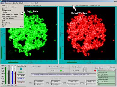
Fig. 17:
Sending data to SPCImage data analysis
SPCImage will come up with the data
contained in the selected window (defined by the corresponding window
intervals). Depending on whether the selected display window was defined for
the laser-off time only or for the whole pixel time SPCImage shows only the
phosphorescence during the laser-off times, or the complete signal, see Fig. 18,
left and right.
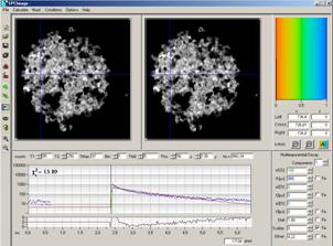
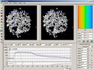
Fig. 18: SPCImage after sending data from SPCM. Left: From a display window
containing data only within Laser-Off intervals. Right: From a display window
containing data of the whole pixel time interval.
The phosphorescence data in Fig. 18, left,
can be analysed without futher preparation. However, analysis will be performed
with an infinitely short instrument response (IRF) width. This will deliver the
correct decay time of a single-exponential phosphorescence decay. However, if
the phosphorescence decay is multi-exponential, the amplitude coefficients of
the decay components cannot be determined correctly.
The data in Fig. 18, right, contain the
combined fluorescence and phosphorescence data. To analyse these data, a
reasonably correct IRF is required. This IRF can be measured, or created as shown
in Fig. 19. Place the cursors of the decay window at the beginning and the end
of the laser-on interval. Then click on the Curve-to-IRF button. This declares
the data in the cursor interval an IRF. The procedure works because (a) the
phosphorescence originates from the S1 population (indicated by fluorescence)
via intersystem crossing and (b) the intensity of the fluorescence during the
laser-on interval is high compared to the intensity of the phosphorescence.
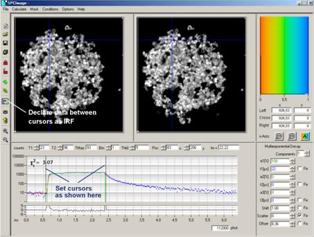
Fig. 19:
Creating an IRF for PLIM analysis
When the IRF has been defined, pull the
right cursor out to the last valid time channel. The rest of the procedure is
the same as for FLIM data [2]. Select the appropriate model parameters on the
right, and click on Calculate, Calculate decay matrix. This starts the
analysis in all pixels of the image. The result is shown in Fig. 20.
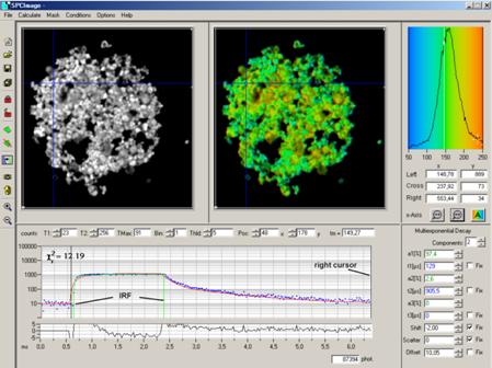
Fig. 20:
Analysed PLIM data
References
1. W. Becker, The bh TCSPC handbook. 4th edition, Becker & Hickl
GmbH (2008), available on www.becker-hickl.com
2.
Becker & Hickl GmbH, Modular FLIM
systems for Zeiss LSM 510 and LSM 710 laser scanning microscopes.
User handbook, available on www.becker-hickl.com
3. W. Becker, B. Su, A. Bergmann, K. Weisshart, O. Holub, Simultaneous Fluorescence and Phosphorescence Lifetime Imaging.
Proc. SPIE 7903 (2011)