Simultaneous Phosphorescence and Fluorescence Lifetime Imaging by Multi-Dimensional TCSPC and Multi-Pulse Excitation

Wolfgang Becker, Stefan Smietana, Becker & Hickl GmbH, Berlin, Germany

Abstract. We present a fluorescence and phosphorescence lifetime imaging (FLIM / PLIM) technique that simultaneously records FLIM and PLIM in confocal or multiphoton laser scanning systems. Different than other techniques, it uses not only one, but multiple laser pulses for every phosphorescence excitation cycle. The sensitivity is thus orders of magnitude higher. Our technique is based on on-off modulating a high-frequency pulsed laser synchronously with the pixel clock of the scanner, and recording the fluorescence and phosphorescence signals by multi-dimensional TCSPC. FLIM is obtained by building up a photon distribution over the times of the photons in the laser pulse period and the scan coordinates, PLIM by building up the distribution over the times of the photons in the laser modulation period and the scan coordinates. The technique does not require a reduction of the laser pulse repetition rate by a pulse picker, and eliminates the need of high pulse energy for phosphorescence excitation.

Motivation of Using Phosphorescence Lifetime Imaging

Phosphorescence occurs when an excited molecule transits from the first excited singlet state, S1, into the first triplet state, T1, and returns from there to the ground state by emitting a photon [24]. Both the S1-T1 transition and the T1-S0 transition are ‘forbidden’ processes. The transition rates are therefore much smaller than for the S1-S0 transition. That means that phosphorescence is a slow process, with lifetimes on the order of microseconds or even milliseconds. Phosphorescence of organic dyes or endogenous fluorophores is extremely weak or even not detectable at room temperature. However, strong phosphorescence with lifetimes from the microsecond up to the millisecond range is obtained for lanthanide complexes [17] and organic complexes of ruthenium [24, 25], platinum [20, 24, 27, 30], terbium, and palladium [27]. Of special interest for live-cell imaging is that the phosphorescence of these complexes is strongly quenched by oxygen. The dyes are therefore excellent oxygen sensors [21, 24, 27, 28, 29, 30, 32]. Applications are aiming at the measurement of oxygen partial pressure in biological objects, and its effect on the metabolism of the cells. To reach this target it is desirable that PLIM and FLIM measurements are performed simultaneously. The oxygen concentration is then derived from the PLIM data, the metabolic information from the FLIM data, preferably from the NAD(P)H fluorescence. To obtain clean FLIM and PLIM data from within cells and tissue the imaging technique must provide depth resolution, and should be able to deliver data from deep tissue layers. The best optical technique to obtain these data is confocal and multiphoton laser scanning, and the best electronic technique to obtain time-resolved data with scanning is multi-dimensional TCSPC [14].

Technical Challenges

Excitation Pulse Period and Laser Power

The obvious problem of PLIM is that the excitation pulse period must be a few times longer than the phosphorescence decay time. For ruthenium dyes with phosphorescence lifetimes below 1 us the reduction in laser repetition rate may still be feasible, see Hosny et al. [25]. However, the lifetimes for platinum and palladium-based dyes are on the order of 50 to 100 µs, and the lifetimes of  europium and terbium dyes can be in the millisecond range. PLIM with these dyes would require a laser repetition rate of less than 10 kHz. Reducing the repetition rate - if possible at all - results in a substantial reduction in the average excitation power, and, consequently, low phosphorescence intensity. Attempts to compensate for the drop in average power by higher peak power are limited by the capabilities of the laser, by saturation and other nonlinear effects in the sample, or, in multiphoton systems, unwanted excitation of higher energy levels or even ionisation. In other words, the effect of reducing the excitation pulse rate is poor sensitivity. Low sensitivity can partially be compensated by high phosphor concentration. However, the commonly used phosphorescence dyes are potentially toxic, and using them in high concentration is not desirable.

Pile-Up Effect

Simply reducing the laser repetition rate causes a significant problem for recording FLIM simultaneously with PLIM. In principle, it would be possible to derive FLIM and PLIM data from a one and the same decay curve that is excited by low-repetition rate laser pulses and simultaneously recorded at two different time scales. One channel would record a photon distribution over the FLIM time scale, the other over the PLIM time scale. However, this would unavoidably create a pile-up problem for the FLIM channel. Typical fluorescence lifetimes are on the order of a few nanoseconds. Neither the detector nor the TCSPC electronics of the FLIM channel are able to detect several photons within this time and determine their arrival times at picosecond accuracy. Detection of several photons per excitation pulse must therefore be avoided. That means the detection rate must be kept at a level no higher than 10% of the excitation rate [10, 12, 13]. With excitation rates on the order of 100 kHz (for Ruthenium) and 10 kHz (for Platinum and Palladium) the available detection rates become extremely low, and, consequently, the acquisition times unacceptably long.

Detector Overload

Another problem is that any sample that emits phosphorescence necessarily also emits fluorescence. The fluorescence both comes from endogenous fluorophores of the sample, and from singlet emission of the phosphorescence probe. At high laser peak power the peak power of fluorescence becomes extremely high. This causes transient overload and extreme afterpulsing in the detectors. It is then impossible to detect a correct phosphorescence decay in the first few microseconds after the laser pulse. In principle, the overload problem can be solved by using laser pulses with a duration in the microsecond range. However, apart from the fact this is not simply feasible with most lasers it would make simultaneous FLIM impossible. More importantly, microsecond pulse duration is not an option for multiphoton excitation.

Interference with Scanning

PLIM in scanning systems has also another problem. The time the scanner stays within the excited sample volume must be longer than the phosphorescence lifetime. If the scanner runs off the excited volume within the phosphorescence decay time photons in the tail of the decay function are lost, and the recorded decay profile gets distorted. Reasonable recording, even of pure intensity images, can thus be obtained only by sufficiently slow scanning. However, if both the pixel time and the pulse repetition period are long there are only a few excitation pulses within the pixel time. Unless the laser pulse sequence is synchronised with the pixel sequence the number of excitation pulses in the pixels varies systematically. This induces Moiré effects in the images. The problem can be solved by synchronising the laser pulses with the pixel frequency, but there is usually no provision for this in normal laser scanning microscopes. Without synchronisation, the pixel time had to be at least 100 times longer than the laser period. This leads to extremely long frame times, and to a further increase of the acquisition time.

Fig. 1: Challenges of PLIM. Left: Low laser repetition rate results in low average excitation intensity. Second left: High peak-to-average power ratio causes high peak intensity of fluorescence, detector overload and afterpulsing, and pile-up in parallel FLIM recording. The phosphorescence intensity remains low due to low average power. Second right: Scanning must be slow enough to stay in the excited pixel over the time of the phosphorescence decay. Right: Low scan rate interferes with low laser pulse repetition rate. This induces Moiré effects in the images.

FLIM - PLIM by Multipulse Excitation

The problems described above are avoided by a FLIM / PLIM technique developed by bh in 2010 [4, 11]. The technique is based on the idea that, if a single short laser pulse is not efficient in exciting phosphorescence, a burst of multiple laser pulses will perform much better. As long as the burst duration is shorter than the phosphorescence lifetime the excitation efficiency will increase in proportion to the number of pulses within the burst. Multi-pulse excitation has been used for multiphoton phosphorescence imaging earlier [30] but bh were first to apply it to TCSPC PLIM.

The principle is shown in Fig. 2. The sample is excited by a pulsed laser running at a repetition rate in the 50 to 80 MHz range, i.e. at a repetition rate as it is typically used for TCSPC FLIM. However, the laser does not run continuously. Instead, it is turned on only for a given period of time, T_on, at the beginning of each pixel. Within the on-time, T_on, the laser pulses excite fluorescence, and, pulse by pulse, build up phosphorescence. The phosphorescence intensity at the end of the laser-on time is far higher than for a single laser pulse.

For the rest of the pixel time the laser is turned off. After the last laser pulse, the fluorescence decays quickly, and for the rest of the pixel dwell time, T_off, pure phosphorescence is detected.

Fig. 2: Principle of Microsecond FLIM. A high-frequency pulsed laser is on-off modulated synchronously with the pixels. FLIM is recorded in the Laser ON phases, PLIM in the Laser OFF phases.

The buildup of TCSPC FLIM and PLIM images with this excitation sequence is straightforward. For each photon, the TCSPC module determines the time, t, within the laser pulse period, and the time, T, after the start of the modulation pulse. The TCSPC process builds up photon distributions over these times and the scan coordinates  [4, 11, 13, 15, 16]

The TCSPC principle is shown in Fig. 3. A fluorescence lifetime image is obtained by building up a photon distribution over the times, t, of the photons in the laser pulse period, and the scanner position, x, y, during the T_on periods. The phosphorescence lifetime image is obtained by building up a similar distribution over the times, T, within the laser modulation period and the beam position, x, y. Thus, fluorescence and phosphorescence lifetime images are obtained simultaneously, in the same scan, and from photons excited by the same laser pulses.

Fig. 3: Simultaneous fluorescence and phosphorescence lifetime imaging

The procedure can be further refined by using the laser on/off information as a routing signal to better separate the fluorescence in laser-on phases from the phosphorescence in the laser-off phases, please see [6, 7, 12].

The principle solves all the problems discussed in the previous section. The excitation pulse rate of FLIM gets de-coupled from the excitation rate of PLIM: The FLIM excitation rate is the laser pulse period, the PLIM excitation period is the period of the on/off modulation. The average excitation intensity drops only by the duty cycle of the laser modulation, and the FLIM excitation rate remains high. High phosphorescence intensity is obtained, and there is no problem with pile-up. The peak intensity of the laser pulses need not be higher than for a normal TCSPC FLIM measurement. The principle thus remains compatible with multiphoton excitation. Moreover, there is no excessively high fluorescence peak intensity, and no detector overload problem. Also the Moiré problem is solved: The laser modulation is automatically synchronised with the pixels of the scan. Every pixel thus gets the same number of excitation pulses.

Implementation in the bh FLIM Systems

All SPC-150, SPC-150N, and SPC‑160 TCSPC module as well as SPC‑830 modules later than serial number 3D0178 (May 2007) [3] have the hardware functions to record simultaneous FLIM / PLIM. The only system requirement is that there is a way to on/off modulate the excitation laser according to the principle shown in Fig. 2. Modulation is performed in different ways in the bh FLIM systems for different laser scanning microscopes.

DCS-120 Confocal Scanning FLIM System

Laser on/off modulation in the DCS-120 system is achieved via the laser multiplexing function of the GVD‑120 scan controller [6]. The system normally has two lasers which can be multiplexed within one pixel. PLIM operation for one laser is obtained by enabling the pixel multiplexing function, and turning the other laser off optically. The laser then turns on at the beginning of each pixel, runs for a fraction of the pixel time, and then turns off.

The parameter definitions are shown in Fig. 4. Both lasers are turned on. The second laser is disabled optically by turning the laser attenuator wheel at the scanner fully down. Laser multiplexing is set to ‘Pixel’. The fraction of the pixel time in which ‘Laser 1’ is on is defined in the field left of ‘% for 1st laser’. This is the time when the laser is running, and fluorescence is measured. For the rest of the pixel time the laser is off, and phosphorescence is measured.

For PLIM, a scan speed must be selected that keeps the scanner within the same pixel for a period of time a few times longer than the phosphorescence decay time. The automatic selection of the scan speed (normally used for FLIM recording) must therefore be turned off, and an appropriate scan speed be selected. This is achieved by turning off the ‘Auto’ button for the scan rate, and selecting a pixel time, T_pxl, a few times longer than the expected phosphorescence decay time.

To avoid that the scanner moves during the pixel time the DCS-120 scanner has an option to run along the lines in steps of the individual pixels (scanners normally run continuously to achieve fast scanning). Stepping along the lines is defined by setting ‘Line Type’ to ‘Steps’.

Scan format and scan area definitions in the scanner control panel are the same as for standard FLIM. Please see [6] for details.

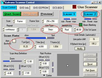
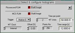
Fig. 4: DCS‑120 scanner setup for simultaneous FLIM/PLIM. Left: Scan and laser control parameters. Right: PLIM timing parameters

The time range of PLIM is defined in the ‘Configure’ sub-menu of the TCSPC system parameters, see Fig. 4, right. For efficient PLIM recording, T_pxl should be a about the same as the ‘Time Range’ selected in the Configure panel. Please see [12] and [6] for details.

DCS-120 MP Multiphoton FLIM System

The DCS-120 MP is the multiphoton version of the DCS‑120 confocal FLIM system. It uses a Ti:Sa laser for excitation [8]. Since November 2015 the DCS‑120 MP is available with a AOM (acousto-optical modulator) for laser power control and modulation. Laser modulation is controlled the same way as for the ps diode lasers of the confocal system. The parameter settings are the same as shown in Fig. 4.

PZ-FLIM-110 Piezo Scanning FLIM System

The PZ-FLIM-110 system uses sample scanning by a piezo stage [9]. Since the stage is driven by the bh GVD-120 scan controller FLIM / PLIM is available the same way as in the DCS-120 system. Please see Fig. 4 for the setup of the scan control parameters.

Zeiss LSM 710, 780, 880 Systems

For the FLIM systems for the Zeiss LSM 710 / 780 / 880 microscope family a bh DDG-210 pulse generator card is added to the FLIM system. The DDG card triggers on the pixel clock of the LSM, and sends a ‘Laser On’ signal to the laser controller of the microscope. The principle is shown in Fig. 5. The pixel clock is split off from the scan synchronisation cable and connected into the trigger input of the DDG card. The ‘Laser On’ signal is connected into the laser control module of the Zeiss LSM via a ‘PLIM’ input. Please note that this input is optional; it has to be ordered from Zeiss via an ‘INDIMO’ (individual modification) request. A PLIM macro has to be installed to activate and de-activate the PLIM input. PLIM Laser control via the DDG‑210 card is integrated in the SPCM software, see Fig. 5, right. The laser-on time is defined on the left. The times on the right define a routing signal that is used to separate the photon from the laser-on and the laser-off times in the SPC module. The routing signal can be delayed with respect to the laser-modulation pulse to compensate for the delay in the AOM of the microscope. Please see [7] for further details.

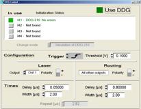
Fig. 5: Left: Principle of laser on/off control for the Zeiss LSMs. Right: Laser control panel of bh SPCM software.

Leica SP5, SP8, SP11 Multiphoton Systems

Since October 2015 FLIM / PLIM is available also for the bh FLIM systems for the Leica SP5, SP8, and SP11 multiphoton microscopes. Laser on-off is controlled by a bh DDG-100 pulse generator module that is added to the FLIM system. The card is triggered by the pixel clock of the microscope. The on-off signal from the DDG is fed into the beam blanking control of the microscope via a logic gate.

Laser power control in the Leica multiphoton systems is performed by an EOM (electro-optical modulator). The EOM is fast enough for PLIM on-off modulation. However, we often found that it does not turn the laser entirely off. This is no problem in standard imaging applications but it can be a problem for PLIM. Spurious excitation during the ‘laser-off’ phases causes a large background in the phosphorescence decay or even makes it impossible to record phosphorescence at all. The solution is an ND filter in the excitation beam path. FLIM / PLIM is performed at no more than 5% of the available laser power. A filter that transmits about 20% shifts the power range from 0 to 5% to 0 to 25%, and reduces the laser power in the off phases sufficiently to avoid spurious excitation. Please use a reflective filter (an absorptive filter may crack), and tilt it by a few degrees to avoid back-reflection into the laser.

Leica systems use a sinusoidal scan in x direction. The nonlinearity of the scan is compensated by a non-uniform pixel time. This is not a problem for the bh FLIM systems: The bh systems use the pixel clock from the Leica scanner and thus avoid distortion of the images [5, 14]. For PLIM, however, the variable pixel time along the lines results in a variable laser on/off period and a variable effective PLIM excitation rate. Also this is not normally a problem. However, the scan rate should be selected slow enough to let the phosphorescence completely decay within the pixel time. Normally, incomplete decay can be taken into account by a suitable model in the SPCImage data analysis [12]. However, this requires that the excitation period is constant over the entire image. This is not the case for PLIM with the Leica microscopes.

Applications

Oxygen sensing

Oxygen sensing by PLIM has become a hot topic in biomedical microscopy, see [21, 24, 27, 28, 29, 30, 32]. Until recently, phosphorescence imaging has mainly been performed by gated camera techniques. The disadvantage of these techniques is that they neither yield images from deeper tissue layers nor images with optical sectioning. PLIM by the technique described here solves these problems by confocal and two-photon laser scanning microscopy, and, additionally, yields FLIM and PLIM simultaneously. An increasing number of publications therefore aims at the use of PLIM for oxygen sensing in cells and tissue. Toncelly et al. used the technique to characterize the sensor dyes [33]. The penetration into cells and the behaviour of the dyes in the biological environment was investigated by Dmitriev et al. [19]. The response of the cells and cell clusters on variations in the oxygen concentration in physiological conditions has been investigated by [18, 22, 23, 29]. An overview on the FLIM / PLIM technique and an introduction into the use of an oxygen-sensitive solid matrix for cells has been given by Jenkins et al. [26].

Examples are shown in the figures below. Fig. 6 and Fig. 7 show cultured human embryonic kidney cells incubated with a palladium-based phosphorescence dye. Fig. 6 was recorded under atmospheric oxygen partial pressure. The maximum of the lifetime distribution over the pixels is at 75 s. Fig. 7 was recorded under decreased oxygen partial pressure. As can be seen, the maximum of the lifetime distribution has shifted to 144 µs.

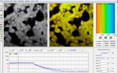
Fig. 6: HEK cells incubated with a palladium dye under atmospheric oxygen partial pressure. Recorded by bh DCS‑120 confocal scanning system, data analysis by bh SPCImage. Lifetime scale 0 (red) to 300 µs (blue). Phosphorescence lifetime at the Cursor-Position 65 µs. The maximum of the lifetime distribution over the pixels is at 75 µs.

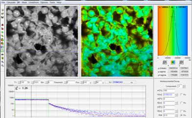
Fig. 7: HEK cells incubated with a palladium dye under reduced oxygen partial pressure. Recorded by bh DCS‑120 confocal scanning system, data analysis by bh SPCImage. Lifetime scale 0 (red) to 300 µs (blue). Phosphorescence lifetime at the Cursor-Position 212 µs. The maximum of the lifetime distribution over the pixels is at 144 µs.

Simultaneous Recording of PO₂ and NAD(P)H Images

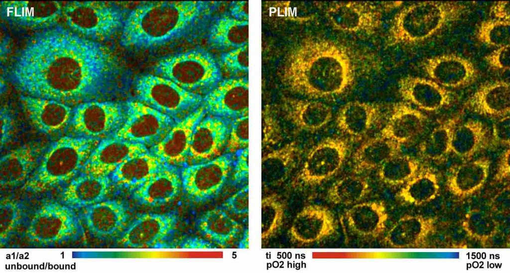
Simultaneously recorded fluorescence and phosphorescence lifetime images of live cultured human squamous carcinoma (SCC-4) cells stained with tris (2,2’-bipyridyl) dichlororuthenium (II) hexahydrate are shown in Fig. 8, left and right. The data were acquired on a Zeiss LSM 780 NLO microscope with a bh Simple-Tau 152 system. The excitation wavelength was 750 nm. The image on the left was recorded in a wavelength interval from 440 to 480 nm. It contains mainly fluorescence of NAD(P)H. The data were analysed with a double-exponential decay model. The image shows the ratio of the amplitudes, a1 and a2, of the decay components. The a1/a2 ratio directly represents the ratio of unbound (a1) and bound (a2) NAD(P)H. The image on the right is the PLIM image. It shows the phosphorescence lifetime of the Ruthenium dye. The lifetime is reciprocally related to the oxygen concentration.

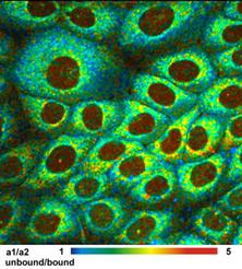
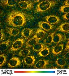
Fig. 8: FLIM and PLIM images of SCC-4 cells stained with (2,2’-bipyridyl) dichlororuthenium (II) hexahydrate. FLIM shown left, PLIM shown right. Zeiss LSM 780 NLO with PLIM option, Simple-Tau 152 FLIM/PLIM system, 2-photon excitation at 750 nm.

Although the results obtained so far look promising caution appears indicated when PLIM data are interpreted in terms of absolute O₂ concentration measurement. As can be seen from Fig. 8 the ruthenium dye binds to the constituents of the cells. The phosphorescence lifetime of bound and unbound dye can be different. Moreover, quenching phenomena are at least in part diffusion-controlled. The quenching rate - and thus the sensitivity to oxygen - more or less depends on the oxygen diffusion constant. The diffusion constant may be different inside the cells and outside, and in different compartments of the cells. pO₂ results derived from PLIM decay times may therefore not necessarily be comparable for different sub-structures of the cells.

Detection of Zinc Oxide Nanoparticles

There are also FLIM / PLIM applications that use phosphorescence to identify nanoparticles in biological tissue, and follow their migration or possible dissolution. The principle is used to track ZnO nanoparticles from sunscreens or cosmetical products in human skin, and investigate possible influence on the viability via the fluorescence of NAD(P)H [31]. Fig. 9 shows zinc oxide nanoparticles can easily be detected by PLIM. The decay function is multi-exponential, with average (intensity-weighted) lifetimes up to 20 µs.

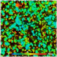
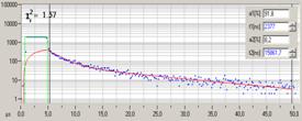
Fig. 9: PLIM of zinc oxide nanoparticles. Left: Lifetime image, intensity weighted lifetime of double-exponential fit. Right: Decay curve at cursor position. Zeiss LSM 710, two-photon excitation at 750 nm, non-descanned detection

PLIM of Inorganic Materials

Fig. 10 was obtained from an Autumit crystal (a uranium mineral). The phosphorescence lifetimes vary from about 100 us to 400 us. The lifetime image is shown on the left, decay curves of two selected spots on the right. The pixel time was 3.6 ms, the laser-on time 200 µs. The excitation wavelength was 405 nm, a 435 nm long pass filter was used in the emission path.

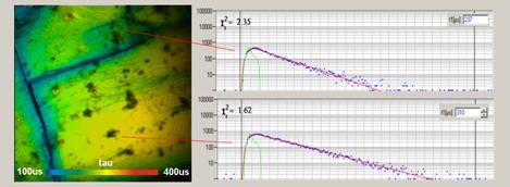
Fig. 10: PLIM image of a uranium mineral. Decay curves if two arbitrary selected spots are shown on the right. 256x256 pixels, 256 time channels, pixel time 3.6 ms, excitation 405 nm, emission filter long pass 435 nm.

Suppression of Autofluorescence

Other applications are using PLIM for suppressing of autofluorescence by using the long lifetime of PLIM as a discrimination parameter [1, 2]. The SPCM software offers this option online, without the need of special data analysis, see [12, 6, 7].

Summary

Compared with PLIM techniques that use a single excitation pulse for every phosphorescence decay cycle our techniques has a number of significant advantages. The first one is that excitation with multiple pulses obtains a significantly higher triplet population than excitation with a single pulse. The sensitivity is therefore much higher. The technique can thus be used at correspondingly lower concentration of the phosphorescence probe, which, in turn, helps reduce possible toxicity. The second advantage is that it is compatible with multiphoton excitation. Due to the excitation with multiple laser pulses it does not require higher laser power or laser pulse energy than normal confocal or multiphoton FLIM. A third advantage is related to the TCSPC technique itself. TCSPC FLIM can record no more than one photon per laser pulse. The photon rate thus has to be limited to no more than 10% of the excitation pulse rate. This is no problem for the 80 MHz or 50 MHz pulse rates of Ti:Sapphire or picosecond diode lasers but it would be a problem if the pulse repetition rate was reduced to the kHz range. Our technique avoids this limitation because it works at the full laser repetition rate. The acquisition times is therefore on the order of 10 to 100 seconds, depending on the expectations to the signal-to-noise ratio of the lifetimes [10, 12]. The only remaining limitation is in the scan rate. The pixel time must not be shorter than about 5 times the phosphorescence decay time. This leads to minimum frame times in the range of 1 second for ruthenium dyes and about 10 seconds for platinum dyes. This no longer than the acquisition time required to obtain the desired signal-to-noise ratio. It thus has no influence on the total acquisition time of the FLIM / PLIM process.

References

1.      E. Baggaley, S. W. Botchway, J. W. Haycock, H. Morris, I. V. Sazanovich, J. A. G. Williams, J. A. Weinstein, Long-lived metal complexes open up microsecond lifetime imaging microscopy under multiphoton excitation: from FLIM to PLIM and beyond. Chem. Sci.   5, 879-886 (2014)

2.      E. Baggaley, M. R. Gill, N. H. Green, D. Turton, I. V. Sazanovich, S. W. Botchway, C. Smythe, J. W. Haycock, J. A. Weinstein, J. A. Thomas, Dinuclear Ruthenium(II) Complexes as Two-Photon, Time-Resolved Emission Microscopy Probes for Cellular DNA. Angew. Chem. Int. Ed. Engl. 53, 3367-3371 (2014)

3.      Becker & Hickl GmbH, FLIM in the FIFO Imaging Mode: Large Images with Small TCSPC Modules. Application note, available on www.becker-hickl.com

4.      Becker & Hickl GmbH, Microsecond Decay FLIM: Combined Fluorescence and Phosphorescence Lifetime Imaging. Application note, available on www.becker-hickl.com

5.      Becker & Hickl GmbH, Multiphoton FLIM with the Leica HyD RLD Detectors. Application note, available on www.becker-hickl.com

6.      Becker & Hickl GmbH, DCS-120 Confocal Scanning FLIM Systems, 6th ed. (2015), user handbook. www.becker-hickl.com

7.      Becker & Hickl GmbH, Modular FLIM systems for Zeiss LSM 710 / 780 / 880 family laser scanning microscopes. 6th ed. (2015), user handbook. available on www.becker-hickl.com

8.      Becker & Hickl GmbH, DCS-120 MP system records multiphoton FLIM and PLIM. Application note (2015), available on www.becker-hickl.com

9.      Becker & Hickl GmbH, PZ-FLIM-110 piezo scanning FLIM system. Data sheet (2015), www.becker-hickl.com

10.   W. Becker, Advanced time-correlated single-photon counting techniques. Springer, Berlin, Heidelberg, New York, 2005

11.   W. Becker, B. Su, A. Bergmann, K. Weisshart, O. Holub,  Simultaneous Fluorescence and Phosphorescence Lifetime Imaging. Proc. SPIE 7903, 790320 (2011)

12.   W. Becker, The bh TCSPC handbook. 9th edition, Becker & Hickl GmbH (2021), available on www.becker-hickl.com

13.   W. Becker, Introduction to Multi-Dimensional TCSPC. In W. Becker (ed.) Advanced time-correlated single photon counting applications. Springer, Berlin, Heidelberg, New York (2015)

14.   W. Becker, V. Shcheslavskiy, H. Studier, TCSPC FLIM with Different Optical Scanning Techniques, in W. Becker (ed.) Advanced time-correlated single photon counting applications. Springer, Berlin, Heidelberg, New York (2015)

15.   W. Becker, Fluorescence Lifetime Imaging Techniques: Time-correlated single-photon counting. In: L. Marcu. P.M.W. French, D.S. Elson, (eds.), Fluorecence lifetime spectroscopy and imaging. Principles and applications in biomedical diagnostics. CRC Press, Taylor & Francis Group, Boca Raton, London, New York (2015)

16.   W. Becker, Fluorescence lifetime imaging by multi-dimensional time correlated single photon counting. Medical Photonics  27, 41-61 (2015)

17.   L.J. Charbonniere, N. Hildebrandt, Lanthanide complexes and quantum dots: A bright wedding for resonance energy transfer. Eur. J. Inorg. Chem. 2008, 3241-3251 (2008)

18.   R. I. Dmitriev, A. V. Zhdanov, Y. M. Nolan, D. B. Papkovsky, Imaging of neurosphere oxygenation with phosphorescent probes. Biomaterials 34, 9307-9317 (2013)

19.   R. I. Dmitriev, A. V. Kondrashina, K. Koren, I. Klimant, A. V. Zhdanov, J. M. P. Pakan,  K. W. McDermott, D. B. Papkovsky, Small molecule phosphorescent probes for O2 imaging in 3D tissue models. Biomater. Sci. 2, 853-866 (2014)

20.   A. Ferchner, S.M. Borisov, A. V. Zhdanov, I. Klimant, D.B. Papkovsky, Intracellular O2 sensing probe based on cell-penetrating phosphorescent nanoparticles. ACS Nano 5 5499-5508 (2011)

21.   H.C. Gerritsen, R. Sanders, A. Draaijer, Y.K. Levine, Fluorescence lifetime imaging of oxygen in cells, J. Fluoresc. 7, 11-16 (1997)

22.   S. Kalinina, V. Shcheslavskiy, W. Becker, J. Breymayer, P. Schäfer, A. Rück, Correlative NAD(P)H-FLIM and oxygen sensing-PLIM for metabolic mapping. J. Biophotonics 9(8):800-811 (2016)

23.   H. Kurokawa, H. Ito, M. Inoue, K. Tabata, Y. Sato, K. Yamagata, S. Kizaka-Kondoh, T. Kadonosono, S. Yano, M. Inoue & T. Kamachi, High resolution imaging of intracellular oxygen concentration by phosphorescence lifetime, Scientific Reports 5, 1-13 (2015)

24.   J.R. Lakowicz, Principles of Fluorescence Spectroscopy, 3rd edn., Springer (2006)

25.   N. A. Hosny, D. A. Lee, M. M. Knight, Single photon counting fluorescence lifetime detection of pericellular oxygen concentrations. J. Biomed. Opt. 17(1), 016007-1 to -12 (2012)

26.   J. Jenkins, R. I. Dmitriev, D. B. Papkovsky, Imaging Cell and Tissue O₂ by TCSPC-PLIM. In: W. Becker (ed.) Advanced time-correlated single photon counting applications. Springer, Berlin, Heidelberg, New York (2015)

27.   A. Y. Lebedev, A. V. Cheprakov, S. Sakadzic, D. A. Boas, D. F. Wilson, Sergei A. Vinogradov, Dendritic Phosphorescent Probes for Oxygen Imaging in Biological Systems. Applied Materials & Interfaces 1, 1292-1304 (2009)

28.   D. Papkovsky, A. V. Zhdanov, A. Fercher, R. I. Dmitriev, and J. Hynes, Phosphorescent oxygen-sensitive probes (Springer, 2012)

29.   D. B. Papkovsky, and R. I. Dmitriev, Biological detection by optical oxygen sensing, Chem Soc Rev 42, 8700-8732 (2013)

30.   S. Sakadžic, E. Roussakis, M. A. Yaseen, E. T. Mandeville, V. J. Srinivasan1, K. Arai, S. Ruvinskaya, A. Devor, E. H. Lo, S. A. Vinogradov, D. A. Boas, Two-photon high-resolution measurement of partial pressure of oxygen in cerebral vasculature and tissue. Nature Methods 7(9) 755-759

31.   W. Y. Sanchez, M. Pastore, I. Haridass, K. König_, W. Becker, M. S. Roberts, Fluorescence Lifetime Imaging of the Skin. In: W. Becker (ed.) Advanced time-correlated single photon counting applications. Springer, Berlin, Heidelberg, New York (2015)

32.   M. Shibata, S. Ichioka, J. Ando, A. Kamiya, Microvascular and interstitial PO2 measurement in rat skeletal muscle by phosphorescence quenching. J. Appl. Physiol. 91, 321-327 (2001)

33.   C. Toncelli, O. V. Arzhakova, A. Dolgova, A. L. Volynskii, N. F. Bakeev, J. P. Kerry, D. B. Papkovsky, Oxygen-sensitive phosphorescent nanomaterials produced from high density polyethylene films by local solvent-crazing. Anal. Chem. 86(3), 1917-23 (2014)

Contact:

Wolfgang Becker

Becker & Hickl GmbH

Berlin, Germany

becker@becker-hickl.com