Shifted-Component Model Improves FLIO Data Analysis

W. Becker, A. Bergmann, Becker & Hickl GmbH, Berlin, Germany

L. Sauer, University of Utah, Salt Lake City, USA

Abstract: We present a new model for analysis of fluorescence-lifetime ophtalmoscopy (FLIO) data. The model uses three exponential components, two of which describe the fundus fluorescence, whereas the third one models the fluorescence of the crystalline lens. The third component is shifted toward short times, accounting for the difference in signal transit time. Compared with the standard triple-exponential model, the fit stability and the lifetime reproducibility are massively improved. Most importantly, the new model allows us to separate the decay components from the fundus from the decay component of the lens. We demonstrate the performance of the new model on FLIO data of a cataract patient who obtained a cataract surgery. Pre-surgery data were dominated by lens fluorescence. Analysed with the conventional three-component model, the data did not deliver useful information about the fundus. With the new model we were able to extract fundus lifetimes which matched the lifetimes from post-surgery images.

Fluorescence-Lifetime Imaging Ophthalmoscopy

TCSPC FLIM is so sensitive that it can be used to record fluorescence-lifetime images of the human retina in vivo. Fluorescence-Lifetime Imaging Ophthalmoscopy, or FLIO, is sensitive to the metabolic state of the tissue. It thus bears the potential to detect early changes in the metabolism of the retina before these have caused irreversible damage. The technique is in use since 1996, and has resulted in an impressive number of research papers [1-35]. FLIO obtained a new push with the introduction of the Heidelberg Engineering FLIO eye scanner, containing bh TCSPC FLIM modules, bh ps diode lasers, and bh HPM hybrid detectors [33, 37]. Fluorescence decay times of the fundus structures range from 200 to 600 ps, with component lifetimes down to less than 80 ps. FLIO data analysis has therefore always been tricky, requiring user interaction and experience to set the fit parameters appropriately. Nevertheless, absolute fluorescence lifetimes obtained by different instruments and different users differed noticeably. This application note analyses the sources of the problem, and presents a new approach which considerably improves the reproducibility of the results.

The Challenges of FLIO Data Analysis

1. The Instrument Response Function (IRF) is not exactly known

The Heidelberg Engineering FLIO (fluorecence-lifetime ophthalmoscope) system records lifetime images of the fundus of the human eye [37]. The decay data contain fluorescence decay components down to less than 100 ps [25]. Under these circumstances, the recorded decay functions are a convolution of the true fluorescence decay functions with the temporal instrument response function (IRF). This is the waveform the system would record for an infinitely short fluorescence decay time [37].

The convolution operation cannot be analytically reversed, i.e. a straightforward de-convolution procedure does not exist. The task is solved by an iterative fit procedure:

- Convolute the model function, _, with the IRF

- Compare result with measured fluorescence data

- Change the model parameters until best fit is obtained

- Repeat the procedure for all pixels of the FLIO data set

Obviously, the IRF has to be known to run this procedure. It is, however difficult, if not impossible, to measure the IRF accurately in a FLIO instrument. A fluorophore with a sufficiently short lifetime (<5ps) and sufficient fluorescence quantum efficiency does not exist. Using a simple scattering target instead faces the problem that the detection system optically blocks the excitation wavelength. To detect the scattered signal modifications have to be made to the optical system, which, in turn, have an influence on the IRF. Moreover, multiple scattering in the target broadens the signal. As a result, the IRF is, if detected at all, recorded broader than it actually is.

2. The optical path length between the scanner and the fundus varies

In FLIO measurements the optical path length from the scanner to the fundus and back is not constant. It depends on the patient's head profile and on the optical length of the eye. Differences of 1 cm in the distance (or 2 cm in the path length) are not unusual. This translates in a transit-time difference of 67 ps. The uncertainty in the transit time results in an uncertainty of the same size in the recorded lifetime [37]. That means lifetimes on the order of 100 ps cannot be determined without shifting the IRF into the correct temporal position.

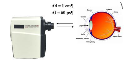
Fig. 1: The path length between the scanner and the eye varies (left). The data analysis has to correct for the associated transit time variation (right).

3. The commonly used model function does not describe the decay profile correctly

The commonly-used model function is a triple-exponential decay of the form

      (1)

This model ignores the fact that the fluorescence from the fundus is overlaid by fluorescence from the crystalline lens. The lens fluorescence arrives 120 to 150 ps before the fundus fluorescence. It not only adds an unwanted decay component to the net decay function in every pixel, it also causes a distortion in the rising edge of the fluorescence pulse (Fig. 2, left). The triple-exponential model (1) is not able to describe the rising edge correctly (Fig. 2, right).

Fig. 2: Left: measured decay function in the presence of lens fluorescence. Right: The model function is not able to describe the rising edge correctly.

The inadequate modelling of the decay funtions in combination with the inaccurately known IRF has consequences:

- The poor fit of the rising edge results in a broad χ2 minimum, ambiguity of the fit, and fit instability.

- There is no clear χ² minimum for different IRF positions. The fit routine is thus unable to find the correct IRF position. Unstable IRF position leads to unstable lifetime results. Moreover, the optimisation procedure tries to compensate for the distortion in the rising edge by modifying the IRF position. Thus, even if an IRF position with minimum χ² is found it is not the correct one.

- The shape of the rising edge depends on the relative amount of lens fluorescence detected. The shape has an influence on the IRF position obtained, and thus on the lifetime determination. As a result, the fundus lifetimes obtained from the fit depend on the focusing, and on the quality of the patient's eye lens, in particular on the amount of astigmatism, and, importantly, on the fluorescence properties of the lens. In particular, there is a problem for cataract patients. These have extraordinarily high lens fluorescence.

It has been attempted to solve these problems by excluding the rising edge from the fit, i.e. by fitting only the part of the decay functions after the maximum. This way, a good χ² is obtained for the falling part of the decay functions. However, the results depend on the selection of the fit range and still contain an uncertainty from the uncertainty of the IRF position. Moreover, fast decay components are not obtained with the best possible accuracy. Information on these components is contained mainly in the early part of the decay functions, i.e. in the part which is excluded from the fit.

The Solution to Accurate FLIO Analysis

1. The Shifted-Component Model

The model function is extended with a parameter, td3, which describes a shift of one of the fluorescence components. The new model function is:

 f(t) = a₁ e^-t/t1 + a₂ e^-t/t2 + a₃ e^(-t+td3)/t3

a1, a2, a3, t1, t2, t3 are fit parameters. t_d3 is the transit time from the lens of the eye to the fundus and back. A model like this has already been suggested by D. Schweitzer [33]. Implementing the model in FLIO data analysis was not successful, however, possibly because the delay was used as a fit parameter. This caused instability of the fit. We therefore assume that t_d3 is constant. In reality, it may vary slightly with the length of the eye. Our tests have shown, however, that the value of t_d3 is not critical. A t_d3 of 120ps to 150ps works well for all adults.

Fig. 3: Modelling the eye fluorescence with the shifted-component model.

The fit delivers two decay components, t₁ and t₂, from the fundus, and a third component, t₃, from the lens. Thus, the shifted component model not only delivers an accurate fit of FLIO data with a correctly positioned IRF, it also allows us to remove the contamination of the fundus data by the lens decay component. This is achieved by calculating an average (amplitude weighted) lifetime, t_m12, only from the first two decay components, t₁ and t₂ and their amplitude factors a₁ and  a₂:

                           (2)

The calculation of t_m12 has been added to SPCImage, see sub-menu 'Colour', 'Encoding of'.

2. Synthetic IRF

We have to accept the fact that it is virtually impossible to measure an accurate IRF for a FLIO system. We therefore defined a mathematical model for the IRF. The model is composed of a term

f(t) = t/t₀·e^-t/t0   describing the temporal response of the detector,

convoluted with

f(t) = e^-(t2/tl)2 describing the shape of laser pulse.

t₀ characterises to detector, t_l the width of the laser pulse. t₀ and t_l are characteristic to each FLIO instrument. They are one-time determined and stored in the instrument software. (An IRF optimisation function is provided in SPCImage but should be used by experts only)

Test of the Shifted-Component Model with a Fast Detector

To test our approach we recorded FLIO data with an HPM-100-06 ultra-fast hybrid detector. The detector itself has an IRF of less than 20 ps full width at half maximum [38], compared to about 120 ps for the HPM-100-40 standard detector [37]. Together with the laser pulse the IRF width is on the order of 40 to 50 ps. With the fast IRF the fit quality can be assessed more accurately than with the standard detector (IRF width about 120 ps). The fact that the fast detector is less sensitive [37] is insignificant for the test. The result is shown in Fig. 4.

The step in the rising edge of the fluorescence (caused by lens fluorescence, compare Fig. 2 and Fig. 3) can easily be seen. It stands out much more prominently than with the standard detectors, where it forms only a kink in the edge. As can be seen in Fig. 4, the model fits the step accurately. The χ2 distribution (shown below the decay curve) is virtually free of bumps in place of the rising edge of the fluorescence pulse.

It should be noted that fitting the data did not require any tweaking of fit conditions or fit-interval boarders. The fit interval was just set to the beginning and the end of the recorded decay data. Small changes in the cursor positions had no visible influence on the results as long as the left cursor remained left of the rising edge and the right cursor in the region where the fluorescence has decayed to reasonably low intensities.

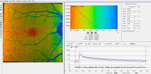
Fig. 4: Test data recorded with ultra-fast hybrid detector. Analysis with shifted component model and syntethic IRF.

Application to FLIO Data of a Cataract Patient

We applied the new analysis approach to data from a cataract patient. The patient obtained a cataract surgery, i.e. got an artificial lens implanted. The natural lens of a cataract eye is highly fluorescent, whereas the artifical one is not. FLIO data were therefore recorded before and after the surgery. The results are shown in Fig. 5 through Fig. 14. All images are shown in normal FLIM style, i.e. with the fluorescence intensity as brightness and the fluorescence lifetime as colour. Opthlamology style is different in that only the lifetime information is shown. We used the normal FLIM style to give an impression of the contrast improvement obtained by the new model. Instructions for SPCImage parameter setup are available in [39].

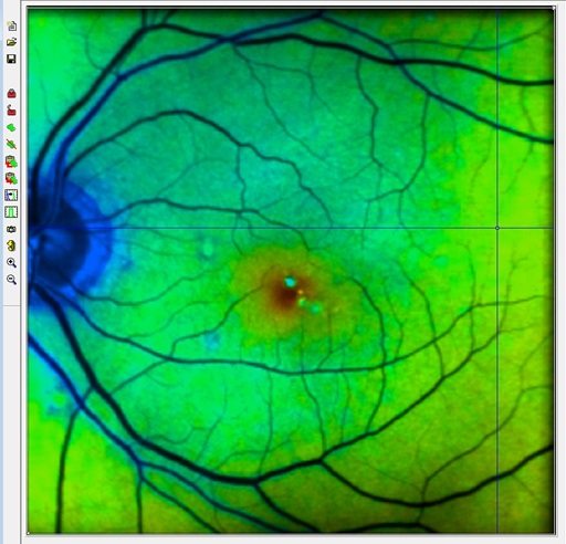
Fig. 5 is a pre-surgery image from the short-wavelength channel with the normal t_m, the amplitude-weighted lifetime of a triple-exponential model. As can be seen from the figure, the lifetime is entirely out of the normal interval of FLO data. The reason is the strong contribution from long-lifetime lens fluorescence.

Fig. 6 is a t_m12 image from the same data set. t_m12 contains only t₁ and t₂, i.e. decay components from the fundus. t_m12 is in the range of normal FLIM data. More interestingly, t_m12 is very close to the t_m  of the post-surgery image, Fig. 11. The post-surgery data contain less or no fluorescence from the lens. The similarity of the lifetimes indicates that t_m12 of the pre-surgery image is really associated with the fundus.

Of course, the large contribution of lens fluorescence has also an effect on the pixel intensities. The lens fluorescence is spatially unspecific, and thus causes a decrease in image contrast. The contrast can be improved by using time-gated pixel intensities from the early part of the decay. This part is dominated by the fundus fluorescence and thus delivers higher contrast. The result is shown in Fig. 7.

A similar, yet less pronounced tendency is found in the pre-surgery images of channel 2 (long wavelength channel). In this wavelength channel the lens fluorescence is weaker than in Channel 1. Nevertheless, the t_m12 image (Fig. 9) shows generally shorter lifetimes than the tm image (Fig. 8). The t_m12 lifetimes are close to the post-surgery t_m lifetimes, see Fig. 13. The gated-intensity image, Fig. 10, has increased contrast, although the improvement is smaller than in channel 1.

Fig. 11 through Fig. 14 are the post-surgery images. Importantly, the t_m lifetimes in the post-surgery images closely match the fundus lifetimes, tm12, in the corresponding pre-surgery images. The t_m12 image in channel 1 of the post-surgery data shows a decay component, t₃, that is clearly associated to the front part of the eye. This is indicated by the kink in rising edge and the perfect it of it. The lifetime is 1.47 ns, compared to 3.64 ns in the pre-surgery data. We do not know where exactly this component comes from but it must be from an anatomic structure in the front part of the eye. There is virtually no such component in channel 2 (long wavelength channel).

Pre-Surgery Images, Channel 1

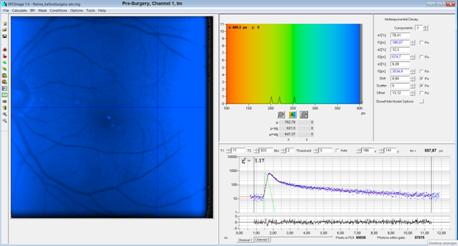
Fig. 5, pre-surgery, tm image: Totally out of normal range, due to lens fluorescence

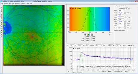
Fig. 6, pre-surgery tm12 image: The lifetime is in the normal range, and close to the post-surgery value. This is an indication that t1 and t2 are indeed fundus-fluorescence components. Note the low contrast due to the strong lens fluorescence.

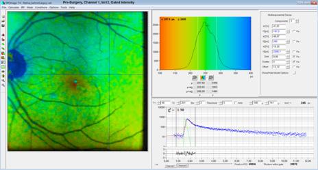
Fig. 7, pre-surgery tm12 image, time-gated intensity: Increased contrast by rejecting most of the lens fluorescence

Pre-Surgery Images, Channel 2

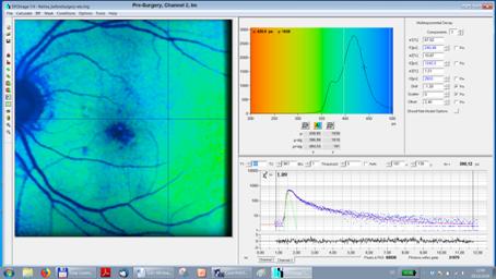
Fig. 8, pre-surgery tm: Lifetime shifted due to lens fluorescence

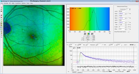
Fig. 9, pre-surgery tm12: The lifetime is close to the post-surgery value (see Fig. 13). This is an indication that t1 and t2 come from the fundus.

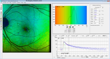
Fig. 10, pre-surgery tm12, gated: Increased contrast by time-gated intensity

Post-Surgery, Channel 1

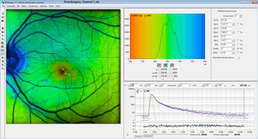
Fig. 11, post surgery tm image. A shifted slow component, t3, is still detected. However, the lifetime (1471 ps) is different than that of the lens (3600ps, see Fig. 6). It probably comes from other anatomic structures of the front part of the eye.

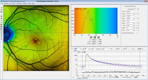
Fig. 12, post surgery tm12 image. In t_m12, the slow component, t₃, is not included. Therefore tm12 is shorter that tm. It is also shorter than tm12 of the pre-surgery image. It is possible that the component is not present in the pre-surgery image, or that it is too week to show up in the pre-surgery data.

Post-Surgery, Channel 2

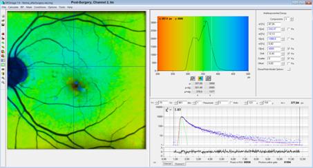
Fig. 13, post surgery tm image. The slow component, t₃, is extremely weak. A trace of a slow component, t₃, turned up only by fixing its lifetime, in this case to 4000ps.

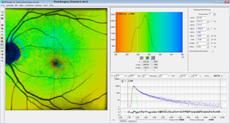
Fig. 14: post surgery tm12 image. Virtually no difference to Fig. 13 because the t₃ component is extremely weak.

Summary

A new model function with a shifted third component in combination with a fully syntethic IRF yields a substantial improvement in the fit stability of FLIO data. We attribute the improvement to the ability of the model to accurately fit the decay component from the front part of the eye. This component is shifted in time and causes a step or a kink in the rising edge of the fluorescence profiles. The accurate fit of the leading part of the decay results in an accurate determination of the temporal position of the IRF. This contributes significantly to the reproducibility of the fit. Moreover, the ability to fit the early part of the decay profiles has a direct influence on the accuracy at which fast fluorescence components are determined. Importantly, the new model allows us the separate the fluorescence decay components of the fundus from the decay component from the lens. This works even for eyes with cataract where the lens is highly fluorescenct. As an additional benefit, FLIO analysis with the new model runs virtually without user interaction. Notably, it does not require tweaking the fit intervals or fit parameters and thus avoids that the results are biased by the operator.

Acknkowledgements

The work described in this note was financially supported by BMBF Germany, project 'Meta Netz'.

References

1.      Karl M. Andersen, Lydia Sauer, Rebekah H. Gensure, Martin Hammer, Paul S. Bernstein, Characterization of Retinitis Pigmentosa Using Fluorescence Lifetime Imaging Ophthalmoscopy (FLIO). TVST 7 No. 3 (2018)

2.      C. Dysli, G. Quellec, M. Abegg, M. N. Menke, U. Wolf-Schnurrbusch, J. Kowal, J. Blatz, O. La Schiazza, A. B. Leichtle, S. Wolf, M. S. Zinkernagel, Quantitative Analysis of Fluorescence Lifetime Measurements of the Macula Using the Fluorescence Lifetime Imaging Ophthalmoscope in Healthy Subjects. IOVS 55, 2107-2113 (2014)

3.      C. Dysli, M.Dysli, V. Enzmann, S. Wolf, M. S. Zinkernagel, Fluorescence Lifetime Imaging of the Ocular Fundus in Mice. IOVS 55, 7206-7215 (2014)

4.      C. Dysli, S. Wolf, K. Hatz, M. S. Zinkernagel, Fluorescence Lifetime Imaging in Stargardt Disease: Potential Marker for Disease Progression. Invest Ophthalmol Vis Sci. 57, 832-841 (2016)

5.      Dysli, C., Wolf, S., Berezin, M.Y., Sauer, L., Hammer, M., Zinkernagel, M.S., Fluorescence lifetime imaging ophthalmoscopy, Progress in Retinal and Eye Research (2017), doi: 10.1016/j.preteyeres.2017.06.005

6.      Dysli, C., Wolf, S., Berezin, M.Y., Sauer, L., Hammer, M., Zinkernagel, M.S., Fluorescence lifetime imaging ophthalmoscopy, Progress in Retinal and Eye Research (2017), doi: 10.1016/j.preteyeres.2017.06.005

7.      C. Dysli, S. Wolf, M.S. Zinkernagel, Fluorescence lifetime imaging in retinal artery occlusion. Invest Ophthalmol Vis Sci. 2015; 56:3329–3336.

8.      C. Dysli, S. Wolf, H.V. Tran, M.S. Zinkernagel, Autofluorescence lifetimes in patients with choroideremia identify photoreceptors in areas with retinal pigment epithelium atrophy. Invest Ophthalmol Vis Sci. 2016;57:6714–6721. DOI:10.1167/ iovs.16-20392

9.      C. Dysli, M. Dysli, M. S. Zinkernagel, V. Enzmann, Effect of pharmacologically induced retinal degeneration on retinal autofluorescence lifetimes in mice. Experimental Eye Research 153 (2016) 178e185

10.   C. Dysli, L. Berger, S. Wolf, M.N S. Zinkernagel, Fundus autofluorescence lifetimes and entral serous chorioretinopathy. Retina 37:2151–2161, 2017

11.   J.A. Feeks, J. J. Hunter, Adaptive optics two-photon excited fluorescence lifetime imaging ophthalmoscopy of exogenous fluorophores in mice. Biomed. Opt. Expr. 8(5), 2483-2495

12.   S. Jentsch, D. Schweitzer, K-U Schmidtke, S. Peters, J. Dawczynski, K-J.n Bär, M. Hammer, Retinal fluorescence lifetime imaging ophthalmoscopy measures depend on the severity of Alzheimer’s disease. Acta Ophthalmologica (2014)

13.   M. Klemm, A. Dietzel, J. Haueisen, E. Nagel, M. Hammer, D. Schweitzer, Repeatability of autoflurescence lifetime imaging at the human fundus in healthy volunteers. Curr. Eye Res. 38, 793-801 (2013)

14.   Kwon S, Borrelli E, Fan W, Ebraheem A, Marion KM, Sadda SR. Repeatability of Fluorescence Lifetime Imaging Ophthalmoscopy in normal subjects with mydriasis. Trans Vis Sci Tech. 2019;8(3):15, https://doi.org/10.1167/tvst.8.3.15

15.   Y. Miura, G. Hüttmann, R. Orzekowsky-Schroeder, P. Steven, M. Szaszak, N. Koop, R. Brinkmann, Two-Photon Microscopy and Fluorescence Lifetime Imaging of Retinal Pigment Epithelial Cells Under Oxidative Stress. IOVS 54 j No. 6, 3369 (2013)

16.   Y. Miura, B. Lewke, A. Hutfilz, R. Brinkmann. Change in Fluorescence Lifetime of Retinal Pigment Epithelium under Oxidative Stress. Nippon Ganka Gakkai Zasshi (J Jpn Ophthalmol Soc) 123,105-114 (2019)

17.   L. Ramm, S. Jentsch, R. Augsten, M. Hammer, Fluorescence lifetime imaging ophthalmoscopy in glaucoma. Graefes Arch Clin Exp Ophthalmol (2014) 252:2025–2026

18.   Lydia Sauer, Rebekah H. Gensure, PhD,1 Martin Hammer, Paul S. Bernstein, Fluorescence Lifetime Imaging Ophthalmoscopy: A Novel Way to Assess Macular Telangiectasia Type 2. Ophthalmology Retina 2 (6), 587-598 (2018)

19.   Lydia Sauer, Rebekah H. Gensure, Karl M. Andersen, Lukas Kreilkamp, Gregory S. Hageman, Martin Hammer, Paul S. Bernstein, Patterns of Fundus Autofluorescence Lifetimes In Eyes of Individuals With Nonexudative Age-Related Macular Degeneration.  IOVS 59 (2018)

20.   S. R. Sadda, E. Borrelli, W.g Fan, A. Ebraheem, K. M. Marion, S. Kwon, Impact of mydriasis in fluorescence lifetime imaging ophthalmoscopy. PLOS ONE | https://doi.org/10.1371/journal.pone.0209194 December 28, 2018

21.   L. Sauer, K.M. Andersen, B. Li, R.H. Gensure, M. Hammer, P.S. Bernstein, Fluorescence Lifetime Imaging Ophthalmoscopy (FLIO) of Macular Pigment. Retina (2018)

22.   L. Sauer, Schweitzer D, Ramm L, Augsten R, Hammer M, Peters S. Impact of macular pigment on fundus autofluorescence lifetimes. Invest Ophthalmol Vis Sci. 2015;56:4668–4679.

23.   Lydia Sauer, Sven Peters, Johanna Schmidt, Dietrich Schweitzer, Matthias Klemm, Lisa Ramm, Regine Augsten, Martin Hammer, Monitoring macular pigment changes in macular holes using fluorescence lifetime imagingophthalmoscopy. Acta Ophthalmologica 2016

24.   Johanna Schmidt, Sven Peters, Lydia Sauer, Dietrich Schweitzer, Matthias Klemm, Regine Augsten, Nicolle Müller,Martin Hammer, Fundus autofluorescence lifetimes are increased in non-proliferative diabetic retinopathy. Acta Ophthalmologica 2016

25.   D. Schweitzer, S. Schenke, M. Hammer, F. Schweitzer, S. Jentsch, E. Birckner, W. Becker, Towards Metabolic Mapping of the Human Retina. Micr. Res. Tech. 70, 403-409 (2007)

26.   D. Schweitzer, M. Hammer, S. Jentsch, S. Schenke, Interpretation of dymanic fluorescence of the eye. Proc. SPIE 677108-1 to -12 (2007)

27.   D. Schweitzer, S. Quick, S. Schenke, M. Klemm, S. Gehlert, M. Hammer, S. Jentsch, J. Fischer, Vergleich von Parametern der zeitaufgelösten Autofluoreszenz bei Gesunden und Patienten mit früher AMD. Der Ophthalmologe 8, 714-722 (2009)

28.   D. Schweitzer, Quantifying fundus autofluorescence. In: N. Lois, J.V. Forrester, eds., Fundus autofluorescence. Wolters Kluwer, Lippincott Willams & Wilkins (2009)

29.   D. Schweitzer, Metabolic Mapping. In: F.G. Holz, R.F. Spaide (eds), Medical retina, Essential in Opthalmology, Springer (2010)

30.   D. Schweitzer, S. Quck, M. Klemm, M. Hammer, S. Jentsch, J. Dawczynski, Zeitaufgelöste Autofluoreszenz bei retinalen Gefäßverschlüssen. Der Ophthalmologe 12, 1145-1152 (2010)

31.   D. Schweitzer, E.R. Gaillard, J. Dillon, R.F. Mullins, S. Russell, B. Hoffmann, S. Peters, M. Hammer, C. Biskup, Time-Resolved Autofluorescence Imaging of Human Donor Retina Tissue from Donors with Significant Extramacular Drusen. IOVS, 53, 3376-3386 (2012)

32.   D. Schweitzer, Autofluorescence diagnostics of ophthalmic diseases. In: V.V. Ghukasyan, A.H. Heikal, eds., Natural biomarkers for cellular metabolism. Biology, techniques, and applications.  CRC Press, Taylor and Francis Group, Boca Raton, London, New York (2015)

33.   D. Schweitzer, M. Hammer, Fluorescence Lifetime Imaging in Ophthalmology. In: W. Becker (ed.) Advanced time-correlated single photon counting applications. Springer, Berlin, Heidelberg, New York (2015

34.   D. Schweitzer, Ophthalmic applications of FLIM. In: L. Marcu. P.M.W. French, D.S. Elson, (eds.), Fluorecence lifetime spectroscopy and imaging. Principles and applications in biomedical diagnostics. CRC Press, Taylor & Francis Group, Boca Raton, London, New York (2015)

35.   D. Schweitzer, L. Deutsch, M. Klemm, S. Jentsch, M. Hammer, S. Peters, J. Haueisen, U. A. Müller, J. Dawczynski, Fluorescence lifetime imaging ophthalmoscopy in type 2 diabetic patients who have no signs of diabetic retinopathy. J. Biomed. Opt. 20(6), 061106-1 to 13 (2015)

36.   J. Teister, A. Liu, D. Wolters, N. Pfeiffer, F.H. Grus, Peripapillary fluorescence lifetime reveals age-dependent changes using fluorescence lifetime imaging ophthalmoscopy in rats. Exp. Eye Res. 176, 110-120 (2018)

37.   W. Becker, The bh TCSPC handbook. Becker & Hickl GmbH, 7th ed. (2017). Available on www.becker-hickl.com

38.   Becker & Hickl GmbH, Sub-20ps IRF Width from Hybrid Detectors and MCP-PMTs. Application note, available on www.becker-hickl.com

39.   FLIO data acquisition and analysis. The road to success. Application note in presentation-style, available on www.becker-hickl.com