DCS-120 Confocal and Multiphoton FLIM Systems

Abstract: The DCS-120 system uses excitation by ps diode lasers, femtosecond fibre lasers or femtosecond titanium-sapphire lasers, fast scanning by galvanometer mirrors, confocal detection, and FLIM by bh’s multidimensional TCSPC technique to record fluorescence lifetime images at high temporal resolution, high spatial resolution, and high sensitivity [1, 2]. The DCS‑120 system is available with inverted microscopes of Nikon, Zeiss, and Olympus. It can also be used to convert an existing conventional microscope into a fully functional confocal or multiphoton laser scanning microscope with TCSPC detection. Due to its fast beam scanning and its high sensitivity the DCS-120 system is compatible with live-cell imaging. The DCS-120 covers the whole range from basic FLIM recording to advanced multi-dimensional FLIM applications. Advanced applications include simultaneous recording of FLIM or steady-state fluorescence images simultaneously in two fully parallel wavelength channels, laser wavelength multiplexing, time-series recording, Z stack FLIM, phosphorescence lifetime imaging (PLIM), fluorescence lifetime-transient scanning (FLITS) and FCS recording. Applications focus on lifetime variations by interactions of fluorophores with their molecular environment. Typical applications are ion concentration measurement, FRET experiments, metabolic imaging, and plant physiology.

DCS-120 Versions for any Kind of Application

The DCS-120 systems are complete laser scanning microscopes for fluorescence lifetime imaging. The systems use bh’s multi-dimensional TCSPC FLIM technology [1, 3, 7, 14, 17] in combination with fast laser scanning and confocal detection or multi-photon excitation [8]. DCS-120 systems are available with various inverted and upright microscopes, see Fig. 1 and Fig. 2. Moreover, the DCS-120 scan head with the associated control and data acquisition electronics can be used to upgrade a conventional microscope with scanning and FLIM recording. In the basic configuration, the DCS-120 uses excitation by two ps diode lasers and records in two parallel detector and TCSPC channels. Advanced versions of the DCS-120 system are available with multiphoton excitation by Ti:Sa lasers and femtosecond fibre lasers (Fig. 2, bottom). The system also works with tuneable excitation sources[29, 30]. A ‘DCS-120 MACRO’ system [1, 9] is available for FLIM of centimetre-size objects, see Fig. 2, second row, right.

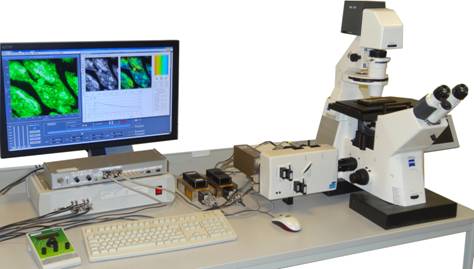
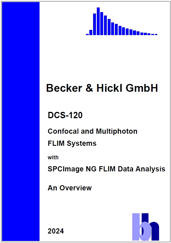
Fig. 1: The DCS‑120 system with a Zeiss Axio Observer microscope

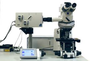
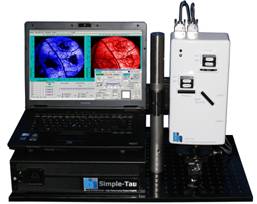
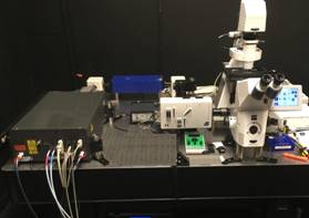
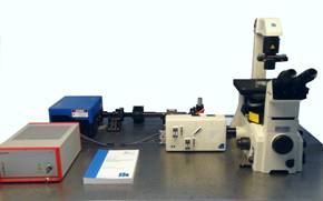
Fig. 2: Upper row: DCS-120 Axio Observer system, DCS‑120 MACRO system. Lower row: DCS-120 MP multiphoton system with Ti:Sa laser, DCS-120 MP multiphoton with femtosecond fibre laser

The DCS systems are using highly efficient GaAsP hybrid detectors, combining extremely high efficiency with large active area, high counting speed, short acquisition time, high time-resolution, and low background [1]. The DCS-120 system is using 64-bit data acquisition software [31], resulting in FLIM at unprecedented pixel numbers. All system components, including lasers, scanner, microscope, and detectors are controlled by one piece of software, making the system easy to use. FLIM data analysis is performed by bh's legendary SPCImage software [5, 4]. It combines time-domain and phasor analysis, uses an MLE algorithm to fit the data, and runs the calculation on a GPU, resulting in data processing times of no more than a few seconds. These features make the DCS-120 system superior to other systems even in entry-level FLIM applications.

However, this is not all. The bh FLIM technique is based on a new understanding of FLIM in general [1]. FLIM is not just considered a way to add additional contrast to microscopy images. Instead, it is considered and designed as a molecular imaging technique. bh FLIM exploits the fact that the fluorescence decay function of a fluorophore is an indicator of its molecular environment, and that multi-exponential decay analysis delivers molecular information, such as the metabolic state of live cells and tissues, protein conformation and protein interaction, reaction of cells to drugs and molecular environment, or mechanisms of cancer development and cancer progression. To reach this target, bh FLIM systems have features not available by other systems: Compatibility with live-cell imaging, extraordinarily high time resolution and photon efficiency, capability to split decay functions into several components, excitation-wavelength multiplexing in combination with parallel-channel detection, recording of dynamic lifetime effects caused by fast physiological effects, and simultaneous FLIM/PLIM [1].

Principle of Data Acquisition

Multi-Dimensional TCSPC

The bh FLIM systems use a combination of bh’s multidimensional time-correlated single-photon counting process with confocal or multiphoton laser scanning. The sample is continuously scanned by a high-repetition rate pulsed laser beam. Single photons of the fluorescence signal are detected, and each photon is characterised by its time in the laser pulse period and the coordinates of the laser spot in the scanning area in the moment of its detection. The recording process builds up a photon distribution over these parameters, see Fig. 3. The photon distribution can be interpreted as an array of pixels, each containing a full fluorescence decay curve in a large number of time channels. In the DCS system, two such recording channels are used in parallel to record images in different spectral intervals or under different polarisation.

Fig. 3: Principle of TCSPC FLIM

The recording process delivers a near-ideal photon efficiency, excellent time resolution, and is independent of the speed of the scanner. The signal-to-noise ratio depends only on the total acquisition time and the photon rate available from the sample.

The technique can be extended by including additional parameters in the photon distribution. These can be the depth of the focus in the sample, the wavelength of the photons, the time after a stimulation of the sample, or the time within the period of an additional modulation of the laser. These techniques are used to record Z stacks or mosaics of FLIM images, multi-wavelength FLIM images, images of physiological effects occurring in the sample, or to record simultaneously fluorescence and phosphorescence lifetime images.

Optical Principle

One-Photon Scanning

The traditional way of laser scanning microscopy is excitation via the traditional one-photon process. That means individual fluorophore molecules are excited by absorbing just one photon of the excitation light at a time. The absorption / emission process is a linear one, i.e. doubled excitation power also induces double emission from the fluorophores. As a result, one-photon excitation excites light in a double cone through the entire depth of the sample, see Fig. 1, left. This causes the commonly known 'out-of-focus blur' in conventional microscopy. To obtain a clean image from a defined focal plane suppression of out-of-focus light is required. The traditional way to solve the problem is laser scanning with 'Confocal Detection'.

Confocal scanning is based on deflecting the excitation beam by fast moving galvanometer mirrors, focusing the beam into the sample via the microscope lens, and feeding the fluorescence from the sample back through the microscope lens and the scan mirrors through a pinhole in a plane conjugate with the focal plane in the sample. Only light from the focal plane passes the pinhole. An image built up by a detector behind the pinhole is free of out-of-focus light and laterally scattered light. Confocal scanning thus delivers extremely clean images of a defined image plane inside an object. This is important especially for FLIM because, once recorded, decay components from unwanted sample planes are hard to remove from the data. The principle of the scanner is shown in Fig. 4.

Two laser beams of different wavelength are coupled into the scanner. They are combined by a beam combiner, pass the main beamsplitter, and are deflected by the scan mirrors. The scan lens sends the beam down the microscope beam path in a way that the scan mirror axis is projected into the back aperture of the microscope lens. The motion of the scan mirrors causes a variable tilt of the beam in the plane of the microscope lens. The laser is thus scanning an image area in the focal plane of the microscope lens. The scanning can be very fast - the line time can be as short as a millisecond, an entire frame can be scanned in less than a second.

Fig. 4: Optical diagram of the DCS-120 scan head. Simplified, see [2] for details

The fluorescence light is collected back through the microscope lens, passes the scan lens, and is again reflected at the scan mirrors. The reflected beam is stationary, independently of the motion of the scan mirrors. It is separated into two spectral or polarisation components, and projected into confocal pinholes. The light signals passing the pinholes are filtered spectrally, and sent to the detectors. Only light from the excited spot in the focal plane of the microscope lens reaches the detectors. The result is a clear image from a defined depth inside the sample which is free of out-of-focus blur and lateral scattering.

MACRO Scanning

The DCS-120 scan head can be used with a wide variety of inverted and upright microscopes of different manufacturers, provided these have an optical port that makes the upper image plane of the microscope lens available. The DCS-120 scan head can, however, also be used without a microscope. In this version of the system, the 'DCS-120 MACRO', the sample is placed directly in the image plane of the scan lens [1, 9]. The system then scans objects as large as 20 mm in diameter.

Fig. 5: DCS-120 MACRO system. It scans a sample directly in the image plane of the scan lens. Samples as large as 20 mm can be scanned.

Multiphoton Scanning

The problem of one-photon excitation is that visible or UV wavelengths have to be used for excitation. The absorption at these wavelengths is high, so that the efficiency decreases rapidly with increasing focus depth in the sample. One-photon scanning therefore cannot be used to image deep layers in biological tissue, see Fig. 6, left. The solution to tissue imaging is multiphoton scanning by a titanium-sapphire laser or a femtosecond fibre laser. Different than confocal scanning, which avoids out-of focus detection, multiphoton scanning avoids out-of-focus excitation. By exciting the fluorophore molecules by a multiphoton (usually two-photon) process only molecules in the focus of the laser are excited, see Fig. 6, middle. Therefore, no pinhole is needed to restrict detection to a defined image plane. The fluorescence light can be fed directly, without passing back through the scanner, to the detectors. This makes it possible to detect fluorescence light which is scattered on the way out of the sample (Fig. 6, right). Moreover, the laser wavelength is in the NIR, where absorption and scattering coefficients are lower than in the visible or UV range. Consequently, deep layers of the sample can be reached. The capability to excite in and detect from deep sample layers makes multiphoton scanning the choice for tissue imaging. Another advantage of multiphoton excitation is that fluorophores with absorption in the UV can be reached without the need of UV optics.

Fig. 6: Comparison of one-photon excitation and multiphoton excitation. Left: The one-photon process excites within a full double cone throughout the sample. The effective excitation power decreases rapidly with increasing depth. Middle: Two-photon excitation excites only in the focus of the laser beam. The NIR laser penetrates deeply into the sample. Right: The fluorescence from a deep focus is scattered on the way out of the sample. It leaves the back aperture of the microscope lens in a wide cone. It cannot be detected via a confocal beam path but very well via NDD.

The principle of the DCS system in the multiphoton configuration is shown in Fig. 7. The beam of a Ti:Sa laser or of a femtosecond fibre laser is fed into the scanner through one of the two laser ports. It can be combined with a visible laser connected to the other port, but this is not a condition for multiphoton operation. The laser beam is deflected by the galvanometer mirrors, and focused in the sample by the scan lens and the microscope lens. The fluorescence light is collected though the microscope lens. However, it is not sent back through the scanner. Instead, it is diverted from the microscope beam path by a dichroic mirror, filtered and/or split into spectral components by a secondary beamsplitter, and fed to one or two detectors. The principle is called 'Non-Descanned Detection'. The FLIM data are built up from the photon pulses of these detectors as described in Fig. 3.

Fig. 7: Scanning with 2-photon excitation. Non-descanned detectors shown on the right.

On-photon excitation, two-photon excitation and descanned and non-descanned detectors can be combined in one DCS-120 system. In that case, a ps diode laser is injected via the second laser port, and the one-photon images are detected by confocal detectors. By enabling either the non-descanned detectors or the confocal detectors the system can be switched from one-photon and multiphoton operation and vice versa.

TCSPC Modules

Different DCS-120 versions can contain different TCSPC / FLIM modules. Early DCS systems used SPC-150 modules. From 2016 on SPC150 N and SPC-150 NX modules were used. The SPC-150 N, and, especially, the SPC-150 NX achieve higher time resolution in combination with ultra-fast hybrid detectors and femtosecond lasers. Recent systems use either the SPC‑180 NX or the SPC-QC-104. The SPC-180 NX delivers maximum time resolution with fast detectors and lasers, the SPC-QC has lower time resolution but can record at extremely high count rates. Still, the instrument response (IRF) of the SPC‑QC 104  is faster than the pulse width of diode lasers and faster than the transit-time spread of most detectors, see Fig. 9. Hence there is little difference in resolution for confocal systems with diode lasers. For systems with femtosecond lasers, however, it can be the difference between easily detecting a fast decay component and missing it.

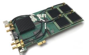
Fig. 8: SPC-180 NX (left) and SPC-QC-104 (right)

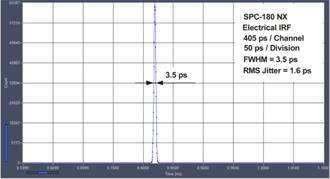
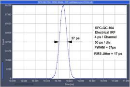
Fig. 9: Electrical IRF for SPC-180 NX (left) and SPC-QC 104

General Features of the DCS-120 System

Precision Confocal and Multiphoton FLIM Images

By using confocal or multiphoton laser scanning and multi-dimensional TCSPC, the DCS system combines the two most precise techniques of recording in space and in time. FLIM images recorded by the DCS-120 systems feature diffraction-limited spatial resolution, ultra-high temporal resolution, suppression of out-of focus fluorescence, suppression of longitudinal and lateral scattering, optical sectioning capability, near-ideal sensitivity and photon efficiency, and low background. By recoding FLIM images with extraordinarily high pixel numbers and time-channel numbers the results are free of undersampling artefacts.

Fig. 10: Megapixel FLIM image recorded by the DCS-120 system. Decay curves in selected pixels on the right.

Ultra-High Efficiency

The bh HPM‑100‑40 GaAsP hybrid detectors of the DCS‑120 combine ultra-high sensitivity with the large active area of a PMT [27]. The large area avoids any alignment problems, and allows light to be efficiently collected through large pinholes and from the non-descanned beam path of the DCS-120 MP system [2]. In contrast to conventional PMTs or SPADs there is no secondary peak or ‘diffusion tail’ in the temporal response. Importantly, the hybrid detectors are free of afterpulsing. The absence of afterpulsing results in improved contrast, higher dynamic range of the decay curves recorded, and in the capability to obtain FCS data from a single detector. The combination of these features makes it easy to detect fluorescence from endogenous fluorophores in single cells and split the decay curves into several decay components, see Fig. 11.

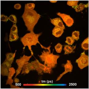
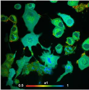
Fig. 11: Autofluorescence lifetime image of NADH in live cells. Lifetime image of mean lifetime of double exponential decay (left)  and image of amplitude of fast decay component, a1 (metabolic indicator, right).

The Ultimate in Time Resolution and Timing Stability

The electrical time resolution of the SPC-180 NX FLIM modules is 3.5ps fwhm, or about 1.5 ps rms [1]. Timing stability is better than 0.4ps rms. The system IRF of a multiphoton system with an HPM-100-06 detector is <19 ps fwhm, or 8.3 ps rms, including detector and laser. Please see Fig. 12. A FLIM example is shown in Fig. 13. The fast decay component, t1, has a lifetime of 10 ps.

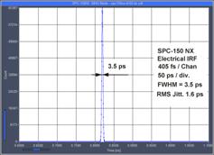
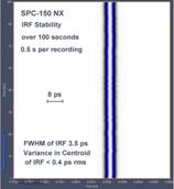
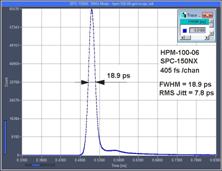
Fig. 12: Electrical IRF, IRF stability, and system IRF with ultra-fast detectors and femtosecond laser excitation

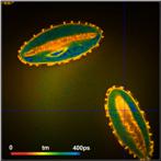
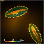
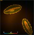
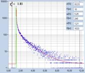
Fig. 13: FLIM of Pollen grains with a dominating decay component of 10 ps. DCS-120 MP, fibre laser, HPM-100-06 fast hybrid detector

Wide Range of Excitation Wavelengths

The DCS-120 confocal system can be used with a wide range of excitation wavelengths. Available diode-laser wavelengths range from 375 nm for excitation of NADH to 785 nm for excitation of NIR dyes. An NADH (autofluorescence) image is shown in Fig. 14, an image of a pig skin sample incubated with 3,3’-diethylthiatricarbocyanine in Fig. 15.

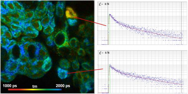
Fig. 14: UV-Excitation FLIM. NADH image of cells, excitation 370 nm, detection 420 to 475 nm.

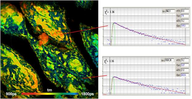
Fig. 15: Near-Infrared FLIM. Pig skin sample stained with 3,3’-diethylthiatricarbocyanine, detection wavelength, excitation 690 nm, detection wavelength from 780 nm to 900 nm.

Fast Beam Scanning - Fast Acquisition

The DCS-120 uses fast beam scanning by galvanometer mirrors. A complete frame is scanned within a time from 100 ms to a few seconds, with pixel dwell times down to one microsecond.

Compared with sample scanning, beam scanning is not only much faster, it avoids also induction of cell motion by exerting dynamic forces on the sample. Moreover, live cell imaging requires a fast preview function for sample positioning and focusing. This can only be provided if the beam is scanned at a high frame rate.

With its fast scanner and its multi-dimensional TCSPC process the DCS system achieves surprisingly short acquisition times. An autofluorescence FLIM image of a live Enchytraeus albidus is shown in Fig. 16. The acquisition time was 1 second. Considering the large pixel number and the high signal-to-noise ratio this is faster than what is achieved by many 'Fast FLIM' techniques [1, 45].

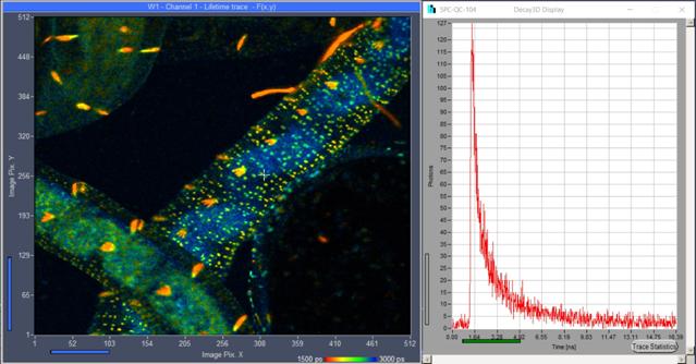
Fig. 16: Lifetime image taken from a live Enchytraeus albidus. Autofluorescence, 1 second acquisition time at 8 MHz average count rate and 80 MHz laser repetition rate. DCS-120 system with SPC‑QC‑104. Online FLIM with SPCM software. Decay curve in selected pixel shown on the right.

Fast scanning also improves the options for time-series recording. The change in the fluorescence lifetime of the chloroplasts in a moss leaf with the time of exposure Fig. 17. Time per image is 1 second.

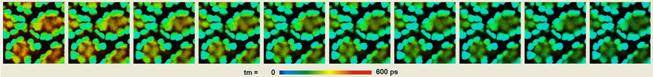
Fig. 17: Change of the fluorescence lifetime of chlorophyll with time of exposure. Moss leaf, excitation at 445 nm, 256 x 256 pixels, 1 image per second.

Megapixel FLIM Images in Two Parallel Channels

With 64 bit SPCM software pixel numbers can be increased to 2048 x 2048 pixels, with a temporal resolution of 256 time channels. The DCS-120 system is able to simultaneously record two high-resolution images in different wavelength or polarisation channels, see Fig. 18 and Fig. 19.

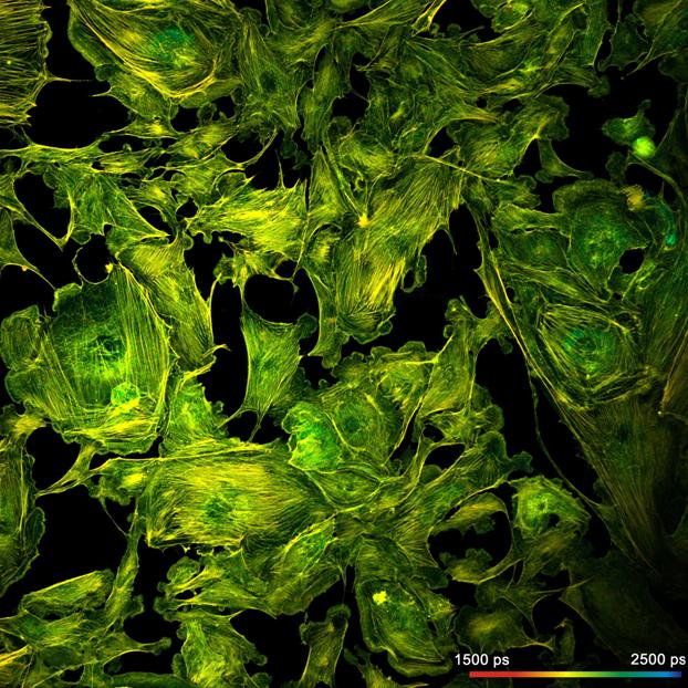
Fig. 18: BPAE sample (Invitrogen) scanned with 2048 x 2048 pixels. Green channel, 485 to 560 nm

Recording is performed in two fully parallel TCSPC channels, avoiding any electronic lifetime or intensity crosstalk. Even if one channel should saturate the other is still producing correct data.

The capability to record images of large pixel numbers is beneficial for a wide range of FLIM applications. One example is tissue imaging where the samples are large, and the images are containing a wealth of detail. It is also useful when a large number of cells have to be investigated and the FLIM results be compared. Megapixel FLIM records images of many cells simultaneously, and under exactly identical environment conditions. Moreover, the data are analysed in a single analysis run, with identical IRFs and fit parameters. The results are therefore exactly comparable for all cells in the image area.

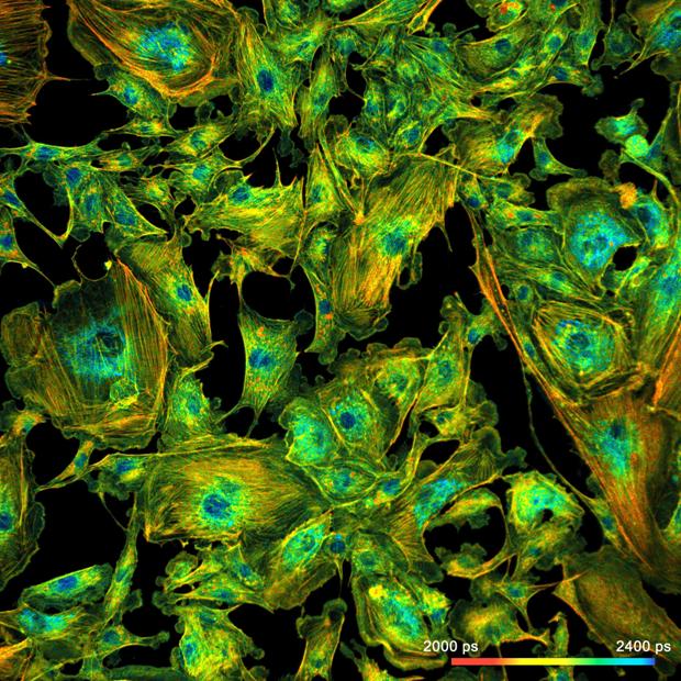
Fig. 19: BPAE sample (Invitrogen), scanned with 2048 x 2048 pixels. Red channel, 560 to 650 nm

High Image Contrast up to the Highest Count Rates

Images taken with conventional TCSPC FLIM at high count rate often suffer from low intensity contrast. The reason is not the pile-up effect, as commonly believed, but intensity nonlinearity by the dead time of the TCSPC process. DCS-120 systems using the SPC-180 or SPC-QC-104 modules do not show this effect. The SPC-180 takes the intensity information from a fast parallel counter with almost no dead time, the SPC-QC-104 avoids dead time by a fast time-conversion method. An image taken at an average count rate of  5.5 MHz is shown in Fig. 20. Peak count rate is about 10 MHz. No loss in contrast by dead time effects is visible.

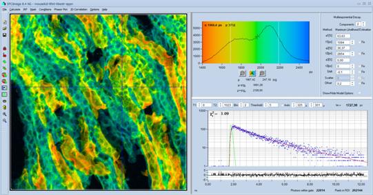
Fig. 20: Image taken at an average count rate of 5.5 MHz. Peak count rate is about 10 MHz. No loss in contrast by dead time effects is visible. DCS-120 with SPC-180 NX module, data analysis by SPCImage NG.

Photon-Counting Intensity Images

A frequently asked question is whether the DCS system can record conventional intensity images. Of course it can - the number of photons, and thus the intensity is part of the FLIM information contained in every pixel of a lifetime image. Recent DCS systems using SPC-180 or SPC-QC-104 TCSPC modules even deliver the intensity without dead-time-induced nonlinearity. Intensity images can be displayed side by side with lifetime images, see Fig. 21.

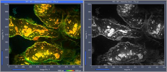
Fig. 21: Lifetime image (left) and intensity image (right), simultaneously displayed by SPCM. SPC-180N, lifetime-intensity mode.

Online Display of Lifetime Images and Decay Curves

The SPCM software is able to display lifetime images and decay curves online during the measurement. Online display of lifetime data helps the user evaluate the quality of the data recorded and, if necessary, restart the measurement in a different region of the sample, with different zoom of the scanner, or with different pinhole size or laser power. An example of online display is shown in Fig. 22.

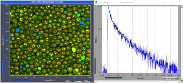
Fig. 22: Online display of lifetime image and decay curve.

Multiphoton FLIM with Ti:Sa Laser

The DCS-120 system is available with multiphoton excitation. The beam of a Titanium-Sapphire laser is fed into one of the laser ports of the DCS scan head. Laser power control and on/off modulation is achieved via an acousto-optical modulator (AOM). Laser control is embedded in the DCS data acquisition software, see 'Software', page 45. FLIM images of pig skin in different depth of the tissue are shown in Fig. 23.

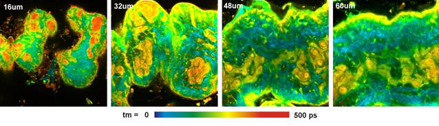
Fig. 23: Pig skin, NADH autofluorescence, image in different depth in the sample. Amplitude-weighted lifetime of triple-exponential decay model

Multiphoton FLIM with Fibre Laser

The DCS-120 can be combined with a femtosecond fibre laser [11, 12]. The preferred wavelength is 780 nm, making the DCS-120 Fibre system perfectly suitable for NADH imaging in tissue. For other fluorophores, the lack of tuneability may be considered a disadvantage. It turns out, however, that most of the commonly used exogenous fluorophores can be excited at reasonable efficiency. This makes the DCS-120 the cheapest multiphoton laser scanning microscope on the market.

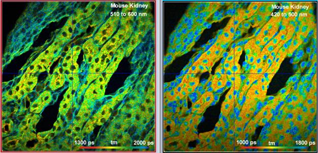
Fig. 24: Mouse kidney sample labelled with Alexa 488, Alexa 568, and DAPI. DCS-120 Fibre, Images simultaneously detected in two spectral channels. Image format 1024 x 1024 pixels, 1024 time channels. Excitation power 3 mW in the sample plane, count rate about 2×10⁶ s­^-1 in each channel.

Non-Descanned Detection

The advantage of multiphoton excitation is that it penetrates deeply into biological tissue. Multiphoton FLIM is therefore the method of choice for molecular imaging in deep tissue. However, fluorescence from deep layers is scattered on its way out of the sample and does not pass back through the scanner.  Therefore its is diverted from the excitation beam path before it re-enters the scanner, and sent to 'Non-Descanned' detectors, please see Fig. 25. Scattered photons from the excited spot are detected by the NDD detectors, and assigned to the current pixel by the TCSPC imaging process. The result is high efficiency for image planes located deeply inside tissue. An example is shown in Fig. 26.

Fig. 25: Principle of non-descanned detection

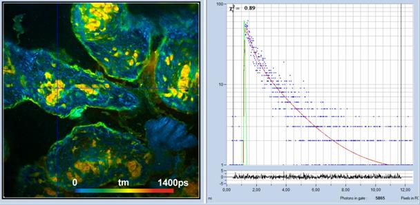
Fig. 26: FLIM of pig skin, NADH image, DCS-120 MP Fibre system, two-photon excitation, non-descanned detection.

Express FLIM

Recording a typical TCSPC image within a short period of time requires an enormous data transfer rate from the TCSPC module to the computer. The data transfer problem increases if a longer sequence of images is to be recorded, and if several TCSPC channels are operated at high count rate simultaneously. bh have solved the problem by a technique called 'Express FLIM'. Express FLIM does not transfer data into the computer photon by photon. Instead, the hardware of the TCSPC module combines the information of all photons within a given pixel into a just two numbers. One is the first moment of the decay curve, the other the number of photons within the pixel. Both numbers are transferred to the computer at the end of each pixel. Even for fast scanning, the required data transfer rate can easily be achieved. The result is a lifetime image that contains first-moment values in the individual pixels. Express FLIM is available for all DCS systems containing the SPC-QC-104 module. An example is shown in Fig. 27.

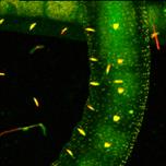
Fig. 27: Express-FLIM of a live Enchytraeus albidus. Autofluorescence, four subsequent images from a 5-frames/second sequence. DCS-120 system with SPC-QC-104. Excitation pulse rate 80 MHz, average photon rate about 10×10⁶ s^-1.

FLIM of Macroscopic Objects

The DCS-120 MACRO system records lifetime images of objects as large as 20 mm in diameter. The system does not use a microscope. Instead, the object is placed directly in the primary image plane of the scanner. For autofluorescence applications the DCS MACRO scan head is available with a scan lens of especially high UV transmission. An example of a MACRO FLIM image is shown in Fig. 28.

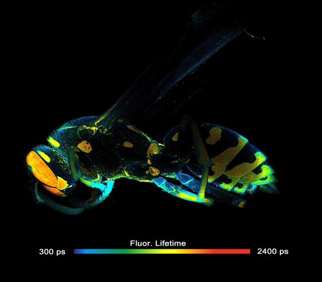
Fig. 28: High-resolution MACRO FLIM image.  2048 x 2048 pixels, 256 time channels per pixel.

FCS

With its time-tag, or, more precisely, parameter-tag mode the DCS-120 confocal system delivers highly efficient FCS. Because the hybrid detectors are free of afterpulsing there is no afterpulsing peak in autocorrelation data [27]. It is not necessary to suppress the afterpulsing peak by cross-correlation, resulting in an increase of the signal-to-noise ratio [1, 16]. An example of FCS is shown in Fig. 29.

Fig. 29: Single molecules diffusing through the laser focus. Decay curve, FCS curve, intensity trace. Raman light suppressed by time-gating. Online fit with FCS procedures of SPCM data acquisition software.

Detection of Nanoparticles

The parameter-tag mode of the DCS system can also be used for single-particle detection. An example for the diffusion of fluorescent nanoparticles through the laser focus in shown in Fig. 30.

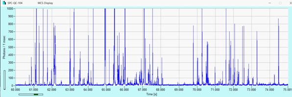
Fig. 30: Fluorescent nanoparticles drifting through the laser focus. Intensity trace.

The individual photon bursts can be further analysed by bh 'SPCDynamics' software, see Fig. 31. SPCDynamics displays fluorescence decay curves integrated over the bursts in a selected time interval, a phasor plot of the decay data of the bursts within a selected time interval, and decay curves and fluorescence lifetimes of individually selected bursts.

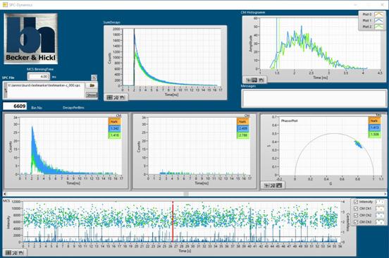
Fig. 31: Analysing photon bursts from single particles or single molecules by bh 'SPCDynamics' software

Recording of Single Decay Curves

The DCS-120 system can record single decay curves from fluorophore solutions or from selected spots in a two-dimensional sample. Curves are obtained either in the 'Single' mode of SPCM, or from summing up the decay data from a pixel area within a FLIM image. This makes a separate lifetime spectrometer for fluorophore characterisation unnecessary. Moreover: A multiphoton system with ultra-fast detectors beats any lifetime spectrometer in time resolution. An example is shown in Fig. 32.

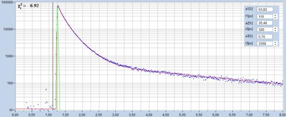
Fig. 32: Fluorescence decay curve recorded with a DCS-120 MP.

Advanced DCS‑120 Functions

Mosaic FLIM

Mosaic FLIM records a large number of consecutive images into a single FLIM data array. The individual images within this array can represent the elements of a tile scan (x-y mosaic), images in different depth in the sample (z-stack mosaic), or images for different times after a stimulation of the sample (temporal mosaic). An example of an x-y mosaic is shown in Fig. 33. The complete data array has 2048 x 2048 pixels, and 256 time channels per pixel. Compared to a similar image taken through a low-magnification lens the advantage of mosaic FLIM is that a lens of high numerical aperture can be used, resulting in high detection efficiency and high spatial resolution.

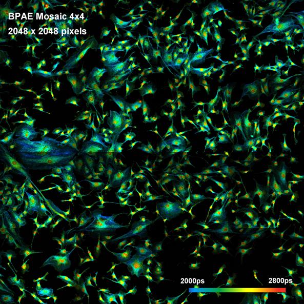
Fig. 33: Mosaic FLIM of a BPAE sample. The mosaic has 4x4 elements, each element has 512x512 pixels with 256 time channels. The entire mosaic has 2048 x 2048 pixels, each pixel holding 256 time channels. DCS‑120 MP multiphoton system with motorised sample stage.

Temporal Mosaic FLIM: Recording of Dynamic Effects

SPCM 64-bit software versions later than 2014 have a ‘Mosaic Imaging’ function implemented. For time-series recording, subsequent frames of the scan are recorded into subsequent elements of the mosaic. The sequence can be repeated and accumulated [1, 8]. The time per mosaic element can be as short as a single frame, which can be less than 100 ms. Another advantage is that the entire array can be analysed in a single SPCImage data analysis run. Fig. 34 shows the change of the lifetime of chlorophyll in plant tissue with the time of illumination.

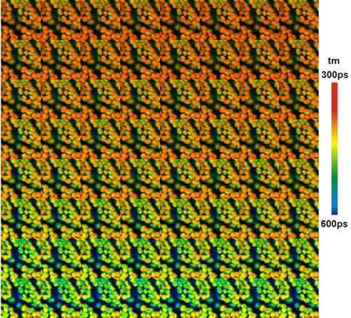
Fig. 34: Time series of chloroplasts in a leaf recorded by Mosaic Imaging. 64 mosaic elements, each 128x128 pixels, 256 time channels. Scan time per element 1s. Experiment time from lower left to upper right. Amplitude-weighted lifetime of double-exponential decay.

Temporal Mosaic FLIM with Triggered Accumulation

When dynamic effects in the fluorescence behaviour of an object are to be recorded the speed is limited by the decrease of the photon numbers in the pixels. The DCS system solves the problem by 'Triggered Accumulation'. A dynamic effect in the measurement object is induced periodically, and the start of the mosaic recording is synchronised with the stimulation. The photon number in the pixels then only depends on the total acquisition time (the number of stimulation periods), and not on the speed of the mosaic recording. As a result, a very fast image sequence can be obtained without the need of exceedingly high photon rate. In fact, triggered accumulation FLIM can be faster than any 'fast FLIM' technique and still be live-cell friendly. An example is shown below.

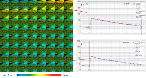
Fig. 35, Left: Calcium transient in cultured neurons, temporal mosaic imaging, 40 ms per image. Image elements 64x64 pixels. bh SPC-150 FLIM system with SPCM software, attached to a Zeiss LSM 7MP microscope.

FLIM of Moving Objects

The recording of fluorescence-lifetime images of live cells or organisms is often impaired by motion in the sample. Nevertheless, the DCS system is able to obtain precision fluorescence-lifetime data from such objects. The technique is based on temporal-mosaic recording and image segmentation by the phasor plot of the bh SPCImage NG data analysis software. A cluster of phasors is selected in the phasor space, identifying pixels of a given decay signature in the FLIM mosaic. These pixels are back-annotated in the mosaic, selecting parts of the objects irrespectively of their location in the individual images. The decay data of the pixels within the selected areas are summed up. The result is a single decay curve with extremely high pixel number which can be analysed at high precision [5, 4].

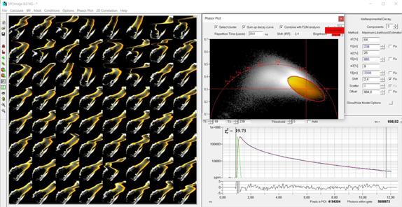
Fig. 36: Precision lifetime analysis on a moving object. A water flee is imaged by temporal mosaic FLIM (left), the phasor range of a structure of interest is selected, and fluorescence-decay analysis is performed on the decay data of the combined pixels within the phasor range.

FLITS: Fluorescence Lifetime-Transient Scanning

FLITS records dynamic effects in the fluorescence lifetime of a sample along a one-dimensional scan. The technique is based on building up a photon distribution over the distance along the scan, the arrival times of the photons after the excitation pulses, and the experiment time after a stimulation of the sample. The maximum resolution at which lifetime changes can be recorded is given by the line scan time. With repetitive stimulation and triggered accumulation transient lifetime effects can be resolved at a resolution of about one millisecond [1, 18, 28,].

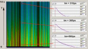
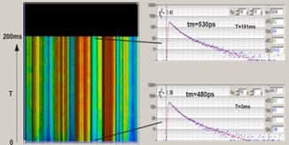
Fig. 37: FLITS of chloroplasts in a grass blade, change of fluorescence lifetime after start of illumination. Left: Non-photochemical transient, transient resolution 60 ms. Right: Photochemical transient. Triggered accumulation, transient resolution 1 ms.

 Z Stack recording

Z stack recording is achieved by controlling the Z drive of the microscope, usually a Zeiss Axio Observer or Axio Examiner, synchronously with the acquisition of an image sequence. The DCS system has two procedures to record Z stacks. One is based on Mosaic FLIM: The data of subsequent planes are recorded in a large FLIM Mosaic. An example of a Mosaic-FLIM Z stack is shown in Fig. 38.

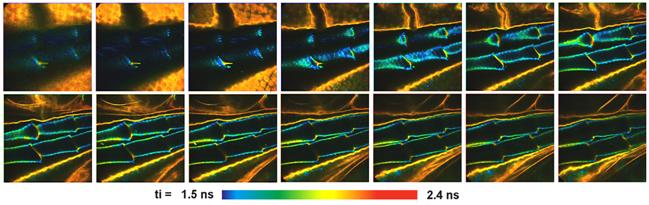
Fig. 38: FLIM Z stack of a part of a water flee. Z stack by mosaic FLIM procedure.

The advantage of Mosaic Z stack recording is that the images of all Z planes are recorded in a single, large FLIM data set. This avoids delay by writing data in subsequent data sets, and guarantees that the data of all planes are exactly comparable. However, the maximum number of planes is limited by the available data space. Depending on the desired lateral resolution, that means that 16 to 64 Z planes can be recorded.

A virtually unlimited number of Z planes can be recorded by a 'record and save' procedure. That means an image of the current plane is recorded, saved into a file, and then the focal plane is moved to the next Z plane. The procedure is repeated until the desired number of planes has been recorded. The record-and-save procedure needs time to save the data but is able to record large number of planes at high x-y resolution. An example of a high-resolution Z stack obtained from a fly, Musca domestica, is shown below. The stack contains 289 planes, each scanned with 1024 x1024 pixels and 1024 time channels. Fig. 39 shows a projection of all planes in a single FLIM image by the 'Multi-File View' of SPCM.

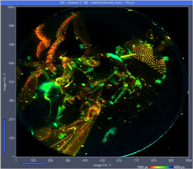
Fig. 39: Vertical projection of all 289 planes of the z stack into a single FLIM image. Planes added by Multi-File View of SPCM, image displayed by Online-Lifetime function of SPCM. Single-exponential lifetime by first-moment analysis.

Fig. 40 shows the same data, analysed by SPCImage and combined into a 3D representation by Image J. All 289 planes were processed with a double-exponential model by the batch-processing function of SPCImage NG, and the resulting 289 tm images written into bmp files by the batch-export function. The bmp files were imported into Image J, which then constructed the 3D representation. For details please see [10].

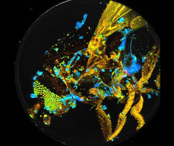
Fig. 40: Decay analysis by SPCImage NG and 3D reconstruction by ImageJ. Colour represents mean lifetime, tm, of double-exponential decay, lifetime range red to blue = 0 to 1250 ps.

Multi-Wavelength FLIM

With the bh multispectral FLIM detectors the DCS‑120 records FLIM simultaneously in 16 wavelength channels [1, 3, 7, 13, 15]. The images are recorded by a multi-dimensional TCSPC process which uses the wavelength of the photons as a coordinate of the photon distribution. There is no time gating, no wavelength scanning and, consequently, no loss of photons in this process. The system thus reaches near-ideal recording efficiency. Moreover, dynamic effects in the sample or photobleaching do not cause distortions in the spectra or decay functions. Multi-wavelength FLIM got an additional push from the new 64-bit SPCM software, and from the introduction of a highly efficient GaAsP multi-wavelength detector [1]. 64-bit software works with enormously large photon distributions, and the GaAsP detector delivers the efficiency to fill them with photons. As a result, 16 images in 16 wavelength channels can be recorded at a resolution of 512x512 pixels and 256 time channels. An example is shown in Fig. 41. For applications please see [1, 37, 47].

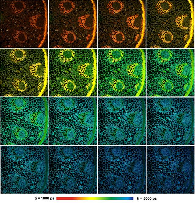
Fig. 41: Multi-wavelength FLIM with the bh MW-FLIM GaAsP 16-channel detector. 16 images with 512 x 512 pixels and 256 time channels were recorded simultaneously. Wavelength from upper left to lower right, 490 nm to 690 nm, 12.5 nm per image. DCS‑120 confocal scanner, Zeiss Axio Observer microscope, x20 NA=0.5 air lens.

It may be suspected that the spatial and temporal resolution of the individual images is mediocre, at best. This is, however, not the case, thanks to the large data space available in the 64-bit environment.   Fig. 42 demonstrates the true spatial resolution of the data. Images from two wavelength channels, 502 nm and 565 nm, were selected from the data shown Fig. 41, and displayed at larger scale and with individually adjusted lifetime ranges. With 512x512 pixels and 256 time channels, the spatial and temporal resolution of the individual images is comparable with what previously could be reached for FLIM at a single wavelength. Decay curves for selected pixels of the images are shown in Fig. 43.

Fig. 42: Two images from the array shown in Fig. 41, displayed in larger scale and with individually adjusted lifetime range. Wavelength channels 502 nm (left) and 565 nm (right). The images have 512 x 512 pixels and 256 time channels.

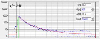
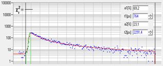
Fig. 43: Decay curves at selected pixel position in the images shown above. Blue dots: Photon numbers in the time channels. Red curve: Fit with a double-exponential model.

Laser Wavelength Multiplexing

Laser multiplexing is used to record FLIM images from fluorophores that cannot be excited at the same wavelength, or the fluorescence of which cannot be discriminated by emission filters. Two, three, or four lasers can be multiplexed in time. Multiplexing is automatically synchronised with the pixels, lines or frames of the scan. The data acquisition software builds up separate images for the individual lasers. An example is shown in Fig. 44. It shows a mouse kidney section, stained with Alexa 488 WGA, Alexa 568 phalloidin, and DAPI. Two excitation wavelengths, 405 nm and 473 nm, were multiplexed. The detection wavelength intervals were 432 nm to 510 nm and 510 nm to 550 nm. Only the combinations of 405 nm with 432 nm to 510 nm and 510 nm to 550 nm, and 473 nm and 510 nm to 550 nm are shown. The fourth combination, 473 nm with 432 nm to 510 nm does not contain reasonable data because the detection interval is too close to the excitation wavelength.

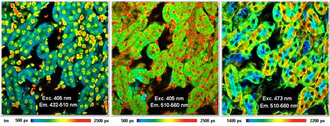
Fig. 44: Excitation wavelength multiplexing, 405 nm and 473 nm. Detection wavelength 432 nm to 510 nm and 510 nm to 550 nm. Mouse kidney section, stained with Alexa 488 WGA, Alexa 568 phalloidin, and DAPI.

Simultaneous FLIM / PLIM

The DCS-120 records FLIM and PLIM by bh's simultaneous FLIM/PLIM technique. The technique is based on on/off modulation of the excitation laser, and recording of lifetime images for the photon times in the laser pulse period and in the laser modulation period [1, 32]. On/off modulation is defined by the laser control parameters. The recording process is synchronised with the modulation via the GVD-120 or -140 Scan controller.

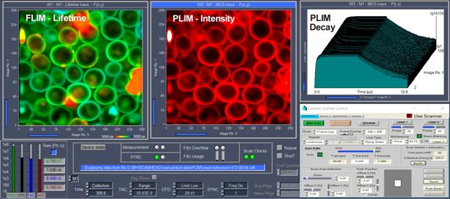
Fig. 45: Simultaneous FLIM / PLIM, main panel of data acquisition software

Applications in Life Sciences

Molecular Imaging

FLIM uses the fluorescence decay function of a fluorophore as an indicator of its molecular environment. The fluorescence decay function, within reasonable limits, neither depends on the fluorophore concentration nor on the excitation power, or other instrumental details. This is a striking advantage over intensity-based imaging techniques. When fluorescence in a sample is excited (Fig. 46, left) the emission intensity (second left) depends not only on possible interaction of the fluorophore with the molecular environment but also on the fluorophore concentration, on possible absorption in the sample, on the excitation power, and on the light collection efficiency of the optics. Changes in the molecular environment can thus not be distinguished from changes in these parameters. Spectral measurements (second right) are able to distinguish between different fluorophores. However, changes in the local environment usually do not cause changes in the shape of the spectrum. The fluorescence lifetime of a fluorophore however (Fig. 46, right), only depends on the fluorophore itself and its interaction the molecular environment.

Fig. 46: Fluorescence. Left to right: Excitation light is absorbed by a fluorophore, and fluorescence is emitted at a longer wavelength. The fluorescence intensity varies with concentration. The fluorescence spectrum is characteristic of the type of the fluorophore. The fluorescence decay function is an indicator of interaction of the fluorophore with its molecular environment.

By using the fluorescence lifetime, or, more precisely, the shape of the fluorescence decay function, molecular effects can therefore be investigated independently of the unknown and usually variable fluorophore concentration [1, 44].

Frequent FLIM applications are ion concentration measurements, probing of protein interaction via FRET, and the probing of the metabolic state and the cell viability via the fluorescence decay parameters of NADH and FAD.

Fluorescence decay functions in these applications are usually multi-exponential. The components of the decay function represent different binding states, different conformations of the fluorophore, or other biologically relevant information. Highly efficient multi-exponential fluorescence-decay analysis is therefore an integral part of the DCS-120 system [4, 5, 6].

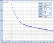
Fig. 47: Real decay function of a fluorophore in biological environment (left) and composition of the curve (right).

Molecular Parameters - Derived from Fluorescence-Decay Data

Molecular environment parameters, such as local pH, ion concentrations, local viscosity or redox potential are available through TCSPC FLIM and precision decay analysis [1]. With appropriate calibration of the probe the results are quantitative, i.e. independent of the laser power, the fluorophore concentration, the parameters of the optical-system, and other instrumental details. Examples are shown below.

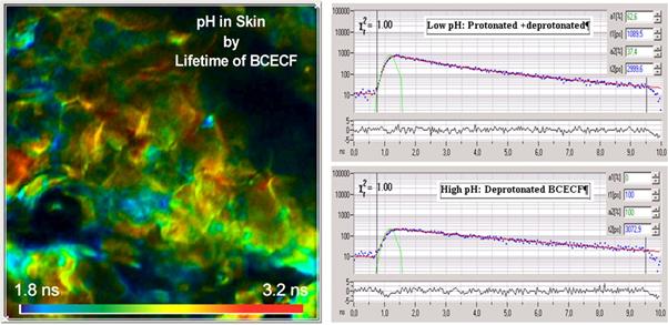
Fig. 48: pH in skin, detected by lifetime of BCECF

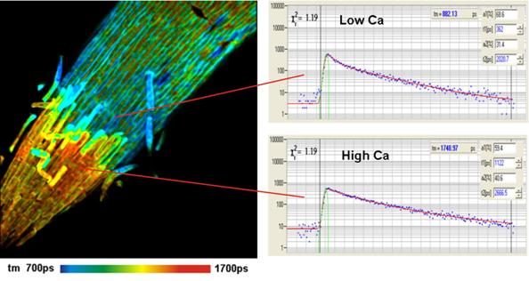
Fig. 49: Calcium concentration in barley root. Detected by lifetime of Oregon Green Bapta

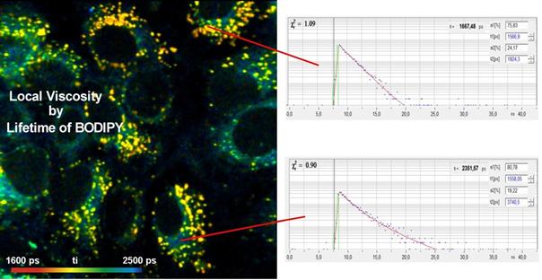
Fig. 50: Local viscosity, detected by lifetime of BODIPY

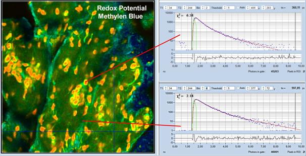
Fig. 51: Redox potential, detected by lifetime of Methylen Blue

FRET - Results from a Single Donor FLIM Image

FRET (Förster Resonance Energy Transfer) is used to probe protein interaction and protein structure in biological systems. The excitation energy is absorbed by a donor. It then transfers to an acceptor, and is emitted via the emission band of the acceptor. The energy transfer occurs only if the distance between the donor and the acceptor is less than a few nm. FRET is used to obtain information about protein interaction, protein folding, and protein structure. FRET experiments by steady-state spectroscopy are difficult to calibrate. FRET is therefore performed mainly by FLIM. But also with FLIM there are problems if the measurement is based on simple single-exponential 'fluorescence lifetimes'. Single-exponential FRET is often considered a quantitative technique but in fact it is not [21].

Quantitative FRET results are only obtained by FLIM in combination with double-exponential FRET analysis. The method has been developed by bh in 2005 and has been constantly improved in the past years. In contrast to single-exponential techniques, the method delivers correct FRET efficiencies and FRET distances even for incomplete donor-acceptor linking, and without reference measurement of a donor-only sample [1, 22]. The classic FRET efficiency, the FRET efficiency of the interacting donor, the amount of interacting donor, and the donor-acceptor distance are displayed directly by SPCImage NG [4]. An example is shown in Fig. 52.

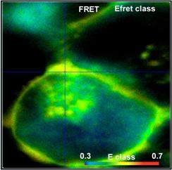
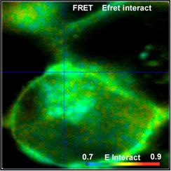
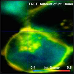
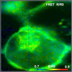
Fig. 52: FRET Measurement in life cell. Classic FRET efficiency, FRET efficiency of interacting donor, amount of interacting donor, and ratio of donor-acceptor distance to Förster radius. bh double-exponential FRET technique, DCS-120 confocal, SPCImage NG data analysis.

FRET-Based Sensors

A large group of sensors for cell parameters is based on FRET. A donor and an acceptor are attached to the ends of a amino-acid linker. The linker changes its conformation with the molecular environment, and so does the fluorescence decay of the donor. For a summary please see FRET chapter in [1]. Fig. 53 shows an open tumor in a mouse, expressing a sensor for apoptosis. The sensor consist of mKate2 (donor) and iRFP (acceptor), connected by an amino-acid linker [48].

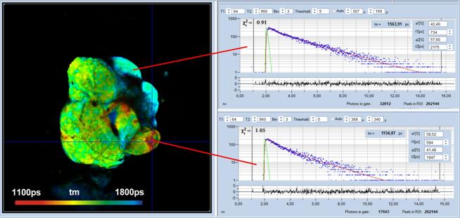
Fig. 53: Open tumor in a mouse, expressing a FRET sensor for apoptosis. DCS-120 MACRO system, analysis by SPCImage NG

Label-Free Imaging

FLIM of Small Organisms

The wide range of excitation and detection wavelengths and the high sensitivity makes the DCS-120 an excellent system for label-free (autofluorescence) FLIM of small organisms. Fig. 54 shows an autofluorescence image of Artemia salinas, a small shrimp living in briny water. A two-photon FLIM image of Artemia salinas recorded by the DCS‑120 MP Fibre system [36] is shown in Fig. 55.

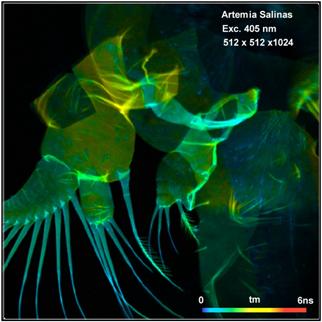
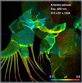
Fig. 54: Autofluorescence FLIM of Artemia salinas. Left: Amplitude-weighted lifetime, tm. Right: Metabolic parameter, a1. DCS-120 confocal system with HPM‑100‑40 hybrid detectors and SPC-180 TCSPC modules, Analysis by SPCImage NG.

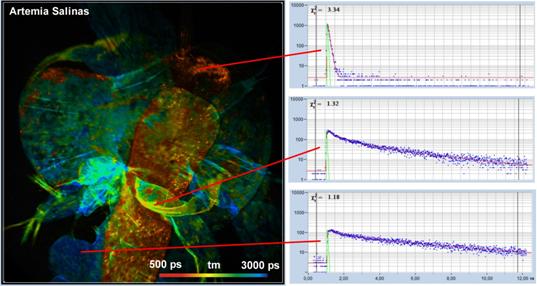
Fig. 55: Two-photon autofluorescence FLIM image of Artemia salinas, mean (amplitude-weighted) lifetime of double-exponential decay. Decay functions of selected areas shown on the right.

Metabolic Imaging by NADH FLIM

For several decades, it has been attempted to obtain metabolic information from the fluorescence lifetime of NADH (nicotinamide adenine dinucleotide). These attempts were not successful in deriving the metabolic state because the lifetimes of the NADH decay components depend also on molecular parameters other than the metabolic state. bh FLIM systems have overcome the problem by using either the amplitude ratio of the decay components (a1/a2) or the amplitude of the decay component of free NADH, a1. It turns out that a1/a2 (the metabolic ratio) or a1 (the metabolic indicator) describe the metabolic state independently of the type of the cell and its molecular environment. Tumor cells have an a1 above 0.7, normal cells an a1 below 0.7. An example is shown in Fig. 56.

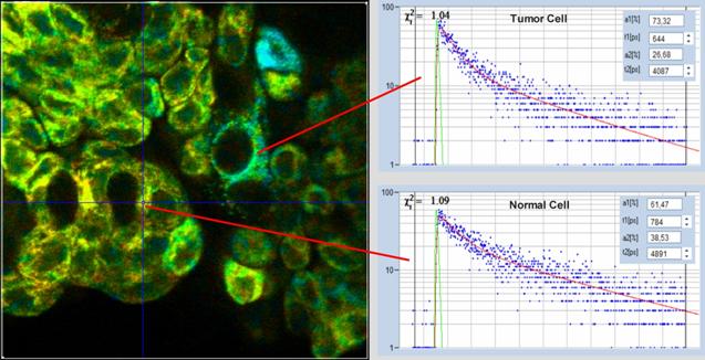
Fig. 56: Metabolic FLIM, a1 image and decay curves. Upper curve: Tumor cell. Lower curve: Normal cell. The tumor cell has an a1 above 0.7. Live human bladder cells from a biopsy. Data analysis with SPCImage NG, MLE algorithm.

NADH FLIM for Clinical Diagnostics

It has been shown that NADH FLIM can be used for clinical diagnostics. FLIM data were obtained from human bladder cells excised during surgery. The patients had been diagnosed with bladder cancer or other suspicious lesions by classic endoscopy. Measurements on the excised material were performed immediately after surgery, before the material went to histology [49]. By using a normal / cancer discrimination threshold of a1 = 0.71 perfect agreement with the histology results was obtained. Please see [1, 19, 20, 49] for details.

NADH FLIM with Multiphoton Excitation and Ultra-Fast Detectors

Metabolic FLIM requires double-exponential data analysis to extract the amplitudes of the decay components of bound and unbound NADH. Separation of the components improves with the time resolution of the FLIM system [34]. The DCS-120 MP multiphoton system in combination with the ultra-fast HPM-100-06 and -07 detectors achieves a time resolution (width of the instrument-response function) of less than 20 ps FWHM [1, 33]. The fast response greatly improves the accuracy at which fast decay components can be extracted from a multi-exponential decay. Date taken with the system not only show the metabolic state of the cells reliably, they also show heterogeneity in the a1 of different mitochondria. An NADH FLIM image recorded with the DCS-120 MP and an HPM-100-06 is shown in Fig. 57. The cells were cultured from a biological cell line. These cells are derived from tumor cells, therefore a1 is larger than 0.7.

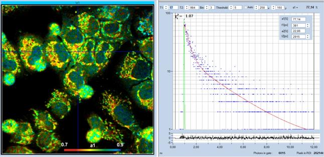
Fig. 57: Left: NADH Lifetime image, amplitude of free NADH, a1. Right: Decay curve at cursor position, 4x4 pixel area. DCS-120 MP with HPM-100-06 detector, FLIM data format 512 x 512 pixels, 1024 time channels. SPCImage NG data analysis.

Metabolic Imaging by simultaneous FLIM of NADH and FAD

When it comes to spectroscopic measurement of the metabolic state often only the fluorescence of NADH is considered. However, also the fluorescence of FAD (flavin adenine dinucleotide) shows a dependence on the metabolic state. Like NADH, FAD exists in a bound and an unbound component. The bound / unbound ratio depends on the metabolic state. The components have different lifetimes, and can be separated by double-exponential decay analysis. The amplitudes of the decay components or the ratio of the amplitudes depend on the metabolic state [2, 1, 46, 50]. Recording FAD FLIM in combination with NADH FLIM may therefore increase the reliability of metabolic imaging. However, there is a problem: The excitation of NADH inevitably also excites FAD, and the fluorescence of FAD cannot be separated from the fluorescence of NADH by emission filtering. The DCS-120 system therefore uses excitation-wavelength multiplexing in combination with dual-channel detection [1, 19], see 'Laser Wavelength Multiplexing', page 30. An example is shown in Fig. 58.

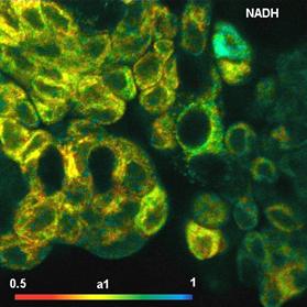
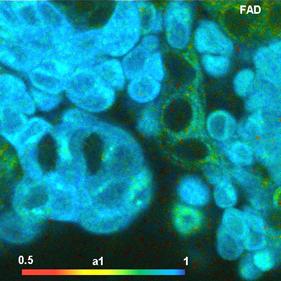
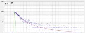
Fig. 58: NADH and FAD images, showing the amplitude of the fast decay component, a1. Same sample as shown in Fig. 56.

Detection of FMN

A problem of using FAD for metabolic imaging is that a part of the fluorescence in the FAD emission range comes from FMN. FNM has a similar emission spectrum as FAD but a different fluorescence lifetime. FMN does not react to the metabolic state the same was as FAD. Therefore its presence can be a problem for quantitative metabolic FLIM. With the high quality of the DCS-120 data and the superior multi-exponential capabilities of SPCImage NG data analysis FAD and FMN can be distinguished in the FLIM data. Fig. 59 shows images of  fractions of bound FAD (a1), free FAD (a2), and FMN (a3) in live human bladder cells.

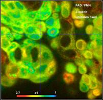
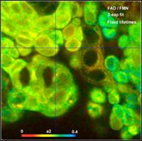
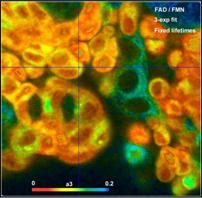
Fig. 59: Amount of bound FAD, free FAD, and FMN in live human bladder cells. Recorded by DCS-120 confocal system.

Label-Free Imaging of Macroscopic Objects

Metabolic FLIM of macroscopic objects is possible with the DCS-120 MACRO system. It differs from the other DCS systems in that the sample is placed directly, without a microscope, in the image plane of the DCS scanner. Objects as large as 20 mm can be imaged in a single scan [1, 9], see Fig. 5, page 7. Fig. 60 shows an NADH image of open tumor in a mouse. Decay curve and decay parameters in selected spots are shown on the right. The metabolic parameter, a1, is 0.61 in the healthy tissue and 0.84 in the tumor. This corresponds well with a1 values from other metabolic FLIM data: a1 is <0.7 in the good tissue and >0.7 in the tumor.

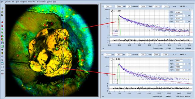
Fig. 60: Open tumor in a mouse, image recorded by DCS-120 MACRO system. Excitation wavelength 370 nm, detection from420nm to 480 nm. The metabolic parameter, a1, is <0.7 in the good tissue and >0.7 in the tumor. This is exactly what is to be expected from other metabolic FLIM experiments.

Ultra-Fast Fluorescence Decay in Biological Material

Due to the short pulse width of the femtosecond lasers the DCS-120 MP system delivers extremely high temporal resolution. An example is shown in Fig. 61. The image shows mushroom spores of Boletus edulis [23]. The image was recorded by a DCS-120 MP with a Femto-Fibre-Pro laser (Toptica), ultra-fast HPM-100-06 detectors, and SPC-150NX TCSPC modules. The data show clearly a decay component of 20 ps lifetime.

An interesting application of ultra-fast FLIM is lifetime imaging of Carotenoids. The lifetimes are in the lower ps range but can easily be resolved by the DCS-120 MP system with ultra-fast detectors [24]. Not only can carotenoids can be localised by their short fluorescence lifetimes, different carotenoids can also be distinguished by different lifetime. Moreover, there are indications that similar carotenoids display different lifetime in different molecular environment. Examples are shown in Fig. 62 and Fig. 63.

Ultra-fast fluorescence decay was also found in human hair and - interestingly - in malignant melanoma. Please see [25] and [26].

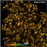
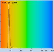
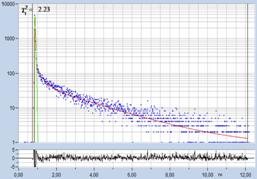
Fig. 61: Spores of Boletus edulis. Left to right: Image of fast decay component, t₁, of triple-exponential decay model, histogram of t₁, and decay curve in selected spot. Data from [23].

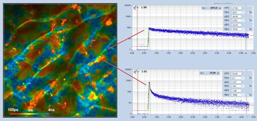
Fig. 62: Lifetime image of carrot tissue. Amplitude-weighted lifetime, tm, of triple-exponential fit. Decay curves in locations without and with b-carotene shown on the right. Triple-exponential decay analysis with SPCImage NG. The fast lifetime component in carotene-rich regions is 8.1 ps.

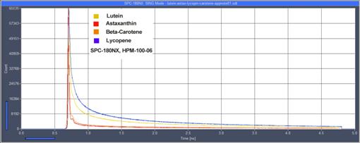
Fig. 63: Decay curves of lutein, astaxanthin, b-carotene, and Lypcopene. Lifetimes are in the range from 10 to 20 ps [24].

Oxygen Sensing by PLIM

Oxygen sensing is based on the quenching of the phosphorescence decay of (exogenous) phosphorescent dyes by oxygen. PLIM can be recorded by the DCS-120 system using triggered MCS recording and multi-pulse excitation [32, 1, 39, 41], see also page 31 of this brochure. Two examples are shown in Fig. 64. The figure shows PLIM images of cultured human embryonic kidney cells incubated with a palladium-based phosphorescence dye. Fig. 64, left was recorded under atmospheric oxygen partial pressure. The maximum of the lifetime distribution over the pixels (upper right) is at 75 µs. Fig. 64, right, was recorded under decreased oxygen partial pressure. As can be seen, the maximum of the lifetime distribution has shifted to 144 µs.

Fig. 64: HEK cells incubated with a palladium dye imaged under different oxygen partial pressure. Left: Atmospheric O2 pressure. Right: reduced oxygen partial pressure. Recorded by bh DCS‑120 confocal scanning system, data analysis by bh SPCImage. Lifetime scale 0 (red) to 300 µs (blue). Phosphorescence lifetime at the Cursor-Position 65 µs. The maximum of the lifetime distribution over the pixels is at 75 µs.

There is currently an increasing interest in PLIM not only for oxygen sensing but also for background-free imaging and luminescence decay of inorganic compounds. In all these applications the bh technique delivers a far better sensitivity than PLIM techniques based on single-pulse excitation.

Simultaneous Sensing of Oxygen and Metabolic State

Oxygen concentration has a large influence of the metabolism of a cell [42, 43]. In fact, the normal / tumor threshold of 0.7 for the metabolic indicator, a1, strictly applies only for oxygen concentrations in the normal physiological range. Consequently, there is large interest to obtain images of the oxygen concentration and the metabolic state simultaneously. This is exactly what the bh FLIM / PLIM technique has been designed for. The technique is based on modulating a ps diode laser synchronously with the pixel clock of the scanner [1, 32]. FLIM is recorded during the ‘On’ time, PLIM during the ‘Off’ time of the laser. The SPCM software delivers separate images for the fluorescence and the phosphorescence which are then analysed with SPCImage NG FLIM/PLIM analysis software [4]. An example is shown in Fig. 65.

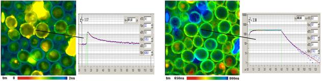
Fig. 65: Yeast cells stained with (2,2’-bipyridyl) dichlororuthenium (II) hexahydrate. FLIM and PLIM image, decay curves in selected spots.

Software

64-bit Data Acquisition Software

The DCS‑120 FLIM systems use the bh SPCM 64 data acquisition software. SPCM runs the data acquisition in the various operation modes of the SPC modules while controlling peripheral devices, such as detectors, lasers, scanners, or motor stages. Operation modes are available for almost any conceivable TCSPC application. There are modes for fluorescence and phosphorescence decay recording, multi-wavelength decay recording, laser-wavelength multiplexing, recording of time series, FCS and photon counting histograms, and there are modes for FLIM, multi-wavelength FLIM, Mosaic FLIM, time-series FLIM, Z stack FLIM, and simultaneous FLIM/PLIM. Since July 2019 SPCM comes with extended multi-threading capabilities, greatly improving the throughput rate even in case of complex online data and display operations. A direct link is provided for communication with SPCImage NG FLIM analysis software.

Since 2013 the SPCM software is available in a 64-bit version. SPCM 64 bit exploits the full capability of Windows 64 bit, resulting in faster data processing, capability of recording images of extremely large pixel numbers, and availability of additional multi-dimensional FLIM modes [1, 31].

The Main Panel of SPCM is configurable by the user [1]. Different configurations can thus be created for different applications and measurement tasks. The configurations can be stored in a Predefined Setup panel and recalled on demand by a single mouse click. A few typical configurations for FLIM systems are shown in Fig. 66. A 154-page description of the SPCM software is available in [1].

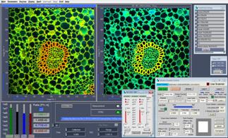
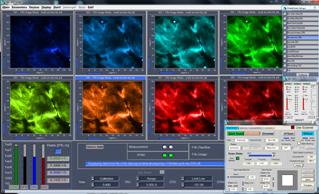
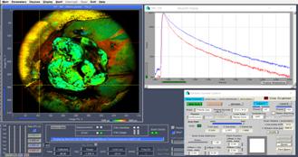
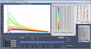
Fig. 66: Main panel of SPCM software. Configurations for dual-channel FLIM, multi-wavelength FLIM, single-channel MCARO FLIM, multi-wavelength curve mode.

Easy Change Between Instrument Configurations

Frequently used instrument configurations are stored in a ‘Predefined Setup’ panel. Changing between the different configurations and user interfaces is just a matter of a single mouse click,  see Fig. 67.

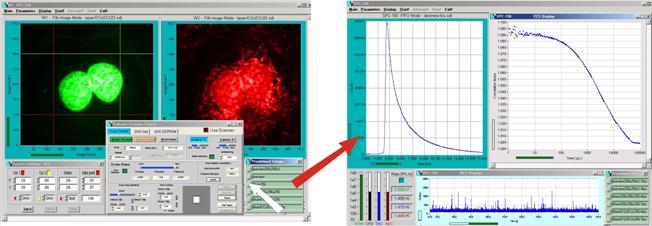
Fig. 67: Changing between different instrument configurations: The DCS-120 system switches from a FLIM configuration into an FCS configuration by a simple mouse click

Integrated Scanner Operation

Scanner control is fully integrated in the data acquisition software. It includes definition of the frame size, pixel numbers, scan speed, and zoom factor. A fast preview mode is provided for sample setup and focus tuning. For a detailed description please see [1] and [2].

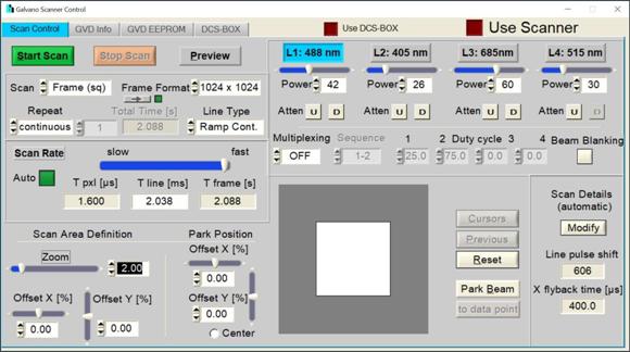
Fig. 68: Scanner Control Panel of the DCS-120 system

Interactive Scanner Control

The zoom factor and the position of the scan area can be adjusted via the scanner control panel or via the cursors of the display window. Changes in the scan parameters are executed online, without stopping the scan. The result becomes immediately visible in the preview images.

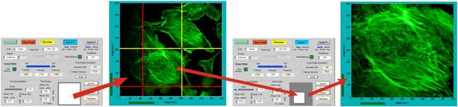
Fig. 69: Interactive scanner control

Automatic Scanner Speed

The DCS-120 scanner control automatically selects the maximum speed of the scanner. Unless otherwise selected, the scanner thus always runs at the highest possible pixel rate, resulting in fast acquisition, minimum triplet excitation, and minimum photobleaching.

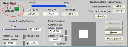
Fig. 70: Automatic selection of scan speed

Integrated Laser Control

Control of up to four lasers is implemented in the scanner control panel. It includes selection of an active laser, beam blanking during the line and frame flyback, intensity control, and laser multiplexing.

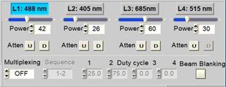
Fig. 71: Laser control part of the scan control panel

Integrated Control of Peripheral Devices

Control of peripheral devices, such as motorised scan stages, Ti:Sa lasers, AOMs for Ti:Sa lasers, or Z drives of microscopes is integrated in the DCS operating software.

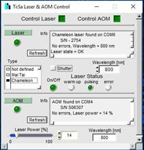
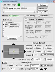
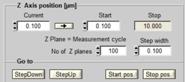
Fig. 72: Control of peripheral devices. Ti:Sa laser and AOM, motorised sample stage, Z drive of Axio Observer

SPCImage NG FLIM Data Analysis

The DCS-120 system uses SPCImage NG FLIM data analysis. SPCImage NG is a new generation of bh's legendary SPCImage TCSPC-FLIM data analysis software. It combines time-domain and frequency-domain analysis, uses a maximum-likelihood (MLE) algorithm to calculate the parameters of the decay functions in the individual pixels, and accelerates the analysis procedure by GPU processing. 1D and 2D parameter histograms are available to display the distribution of the decay parameters over the pixels of the image or over selectable ROIs. Image segmentation can be performed via the phasor plot. Pixels with similar phasor signature can be combined for high-accuracy time-domain analysis. SPCImage NG provides decay models with one, two, or three exponential components, incomplete-decay models, and shifted-component models. Another important feature is advanced IRF modelling, making it unnecessary to record IRFs for the individual FLIM data sets. For a detailed description please see [1, 2, 4], and SPCImage NG Overview Brochure [5]. A typical main panel of SPCImage NG is shown in Fig. 73.

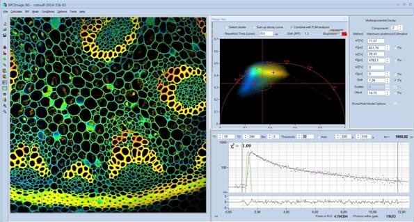
Fig. 73: Example of SPCImage NG main panel. Combination of time-domain analysis (left and lower right) and phasor plot (upper right)

Deconvolution and Fit Procedure

SPCImage NG runs an iterative fit and de-convolution procedure on the decay data of the individual pixels of the FLIM images. In the simplest case, the result is the lifetime of the decay functions in the individual pixels. For complex decay functions the fit procedure delivers the lifetimes and amplitudes of the decay components. SPCImage then creates colour-coded images of the amplitude- or intensity-weighted lifetimes in the pixels, images of the lifetimes or amplitudes of the decay components, images of lifetime or amplitude ratios, and images of other combinations of decay parameters, such as FRET intensities, FRET distances, bound-unbound ratios, or the fluorescence-lifetime redox ratio, FLIRR. A few examples are shown in Fig. 74 and Fig. 75. For details please see [1, 2, 4].

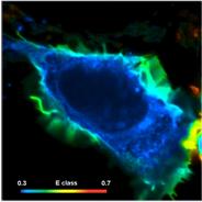
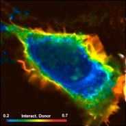
Fig. 74: Cell with interacting proteins, labelled with a FRET donor and a FRET acceptor. Left to right: Classic FRET efficiency, fraction of interacting donor, FRET distance

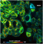
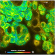
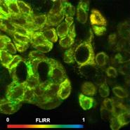
Fig. 75: Metabolic FLIM. Bound-unbound ratio of NADH, Bound/unbound ratio of FAD, Fluorescence-Lifetime Redox Ratio, FLIRR.

GPU Processing

SPCImage NG uses GPU (Graphics Processor Unit) processing. GPU processing is running on NVIDIA cards and a number of other NVIDIA-compatible devices. The TCSPC data are transferred into the GPU, which then runs the de-convolution and fit procedure for a large number of pixels in parallel. This way, data processing times for large images are reduced from formerly more than 10 minutes to a few seconds.

Maximum-Likelihood Algorithm

Unlike earlier SPCImage versions, SPCImage NG uses a maximum-likelihood algorithm (or maximum-likelihood estimation, MLE) for fitting the data. In contrast to the usual least-square fit, the MLE algorithm takes into account the Poissonian distribution of the photon numbers. Compared to the least-square method, the fit accuracy is improved especially for low photon numbers, and there is no bias toward shorter lifetime as it is often observed for the least-square fit. For comparison with older data sets the weighted least-square fit and the first-moment algorithms of the previous SPCImage versions are still available in SPCImage NG.

Instrument-Response Function

SPCImage NG avoids troublesome recording of an instrument response function (IRF) for each FLIM measurement. This is achieved by modelling the IRF with a generic function. The parameters of this function are determined by fitting it to the FLIM data together with the selected decay model. The results of this procedure are so good that an accurate IRF is obtained even for decay functions containing ultra-fast components, see Fig. 76. For details please see [4].

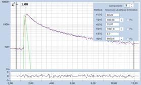
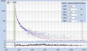
Fig. 76: Synthetic IRF. Left: Autofluorescence of cells, ps diode laser, HPM-100-40. Right: Sample with extremely fast decay component, femtosecond fibre laser, HPM-100-06

Phasor Plot

SPCImage NG combines time-domain multi-exponential decay analysis with a phasor plot. In the phasor plot, the decay data in the individual pixels are expressed as phase and amplitude values in a polar diagram [38]. Independently of their location in the image, pixels with similar decay signature form clusters in the phasor plot. Different phasor clusters can be selected, and the corresponding pixels back-annotated in the time-domain FLIM images. The decay functions of the pixels within the selected phasor range can be combined into a single decay curve of high photon number. This curve can be analysed at high accuracy, revealing decay components that are not visible by normal pixel-by pixel analysis [4, 35]. An example is shown in Fig. 77.

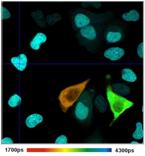
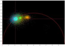
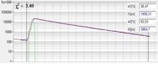
Fig. 77: Combination of time-domain analysis with phasor plot. Left to right: Lifetime image, phasor plot, decay curve of combined pixels within selected phasor range

Image Segmentation

SPCImage NG provides automatic image segmentation functions via the phasor plot and 2D histograms of the decay parameters. Areas with different decay signature form separate clusters in these presentations. Interesting clusters can be selected and back-annotated in the images. The decay data of the corresponding pixels are combined into a single decay curve with extremely high photon number. Multi-exponential decay analysis on the combined data delivers precision decay parameters even if the photon numbers in the individual pixels are low. An example is shown in Fig. 78.

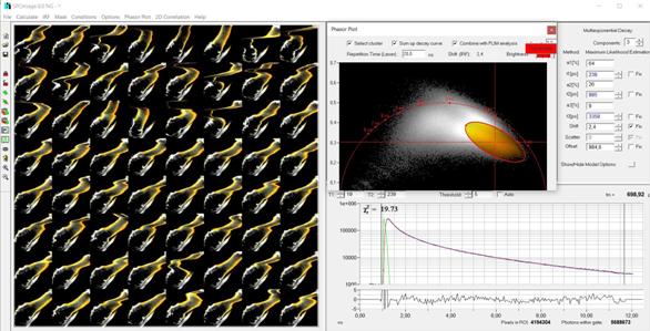
Fig. 78: Image segmentation on temporal-mosaic FLIM data of a live water flee

Single-Curve Analysis

SPCImage can also be used to analyse single decay curves, The data can come from traditional cuvette experiments, or from the combined pixels of a FLIM recording. An example is shown in Fig. 79.

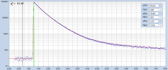
Fig. 79: SPCImage used for fluorescence decay analysis of single curves. NADH dissolved in water, recorded with bh DCS-120 MP FLIM system.

Summary

The DCS-120 is a high-performance lifetime imaging system based on laser scanning and multi-dimensional TCSPC. The system is characterised by high time resolution, high sensitivity, high photon efficiency, high spatial resolution, and suppression of out-of-focus fluorescence and laterally and longitudinally scattered light. The system comes in different versions: The standard DCS-120 system uses excitation by ps diode lasers and confocal detection, the DCS-120 MP systems use multiphoton excitation and non-descanned detection. The DCS-120 MP Fibre uses a femtosecond fibre laser for excitation, making it the cheapest multiphoton microscope on the market. All systems can be delivered as complete laser scanning microscopes or as FLIM upgrades for existing conventional microscopes. Moreover, there is the DCS-120 MACRO system for scanning cm-size objects directly in the primary image plane of the scanner.

The DCS system can be used for the whole range of FLIM applications: From entry-level to high end molecular imaging. The DCS-120 is based on a new understanding of FLIM in general.

Different than other FLIM techniques and FLIM systems which consider FLIM just a way to improve contrast in laser scanning microscopy, the DCS-120 has been designed with molecular-imaging applications in mind. It thus has capabilities beyond the reach of other systems: Compatibility with live-cell imaging, extraordinarily high time resolution and photon efficiency, capability to split decay functions into several components, excitation-wavelength multiplexing in combination with parallel-channel detection, recording of dynamic lifetime effects caused by fast physiological effects, and simultaneous FLIM/PLIM. Typical applications are measurement of molecular-environment parameters, protein-interaction experiments by FRET techniques, label-free imaging, imaging of the metabolic state of cells and tissues, the use of endogenous fluorophores with lifetimes in the 10-ps range, oxygen-concentration measurement, and recording of fast physiological processes in biological systems. No other FLIM technique and no other FLIM system offers a similar range of advanced capabilities.

Specifications

Scan head                                                                                     bh DCS-120 scan head

Optical principle                                                        confocal, beam scanning by fast galvanometer mirrors

Laser inputs                                                                 two independent inputs, fibre coupled or free beam

Laser power regulation, optical                                  continuously variable via neutral-density filter wheels

Outputs to detectors                                                            two outputs, detectors are directly attached

Main beamsplitter versions                                                multi-band dichroic, wideband, multiphoton

Secondary beamsplitter wheel     3 dichroic beamsplitters, polarising beamsplitter, 100% to channel1, 100% to channel2

Pinholes                                                                            independent pinhole wheel for each channel

Pinhole size                                                                            11 pinholes, from about 0.5 to 10 AU

Emission filters                                                                                2 filter sliders per channel

Connection to microscope                                          adapter to left side port or port on top of microscope

Coupling of lasers into scan head (visible)              single-mode fibres, Point-Source type, separate for each laser

Coupling of laser into scan head (Ti:Sa)                                      free beam, 1 to 2 mm diameter

Scan Controller                                                                                   bh GVD-120

Principle                                                        Digital waveform generation, scan waveforms generated by hardware

Scan waveform                                                                          linear ramp with cycloid flyback

Scan format                                                                                     line, frame, or single point

Frame size, frame scan                                                                   16x16 to 4096x4096 pixels

                     line scan                                                                            16 to 4096 pixels

Laser power control, electrical                                                       via electrical signal to lasers

Laser multiplexing                                                         frame by frame, line by line, or within one pixel

Beam blanking                                                                     during flyback and when scan is stopped

Scan rate                                                                    automatic selection of fastest rate or manual selection

minimum pixel time for frame size              64x64      128x128    256x256       512x512     1024x1024   2048x2048

                       Zoom=1                                25.6µs       12.8µs        6.4µs            3.2µs            1.6µs            1.2µs

                       Zoom=8                                 6.4µs         3.2µs         1.6µs            0.8µs            0.6µs            0.5µs

minimum frame time for frame size             64x64      128x128    256x256       512x512     1024x1024   2048x2048

                       Zoom=1                                 0.19s         0.37s         0.64s            1.24s             2.6s              6.5s

                       Zoom=8                                0.037s       0.074s       0.173s          0.320s            1.0s              2.7s

Scan area definition                                       via zoom and offset or interactive via cursors during preview

Fast preview function                                                       1 second per frame, 128 x 128 pixels

Beam park function                                              via cursor in preview image or cursor in FLIM image

Laser control                                                     2 Lasers or 4 Lasers, on/off, frame, line, pxl multiplexing

Diode lasers                                                                                  BDS-SMN laser

Number of lasers simultaneously operated                                                   2

Wavelengths                                        375nm, 405nm, 445nm,  473nm, 488nm, 510nm, 640nm, 685nm, 785nm 

Pulse width, typical                                                                               30 to 70 ps

Pulse frequency                                                                      20MHz, 50MHz, 80MHz, CW

Power in picosecond mode                      0.25mW to 1mW injected into fibre. Depends on wavelength version.

Power in CW mode                                     10 to 40mW injected into fibre. Depends on wavelength version.

Other lasers

Visible and UV range                                            any ps pulsed laser of  20 to 80 MHz repetition rate

     Coupling requirements                                         Point-Source Kineflex compatible fibre adapter

     Wavelength                                                                any wavelength from 400nm to 800nm

fs NIR Lasers for multiphoton operation                                              any fs laser

     Coupling requirements                                                      free beam, diameter 1 to 2 mm

     Wavelength                                                                                  700 to 1200 nm

Detectors (standard)                                                        bh HPM-100-40 hybrid detector

Spectral Range, incl. DCS optics                                                         330 to 710nm

Peak quantum efficiency                                                                       40 to 50%

System IRF width with bh diode laser                                                 120 to 130 ps

System IRF with fs laser                                                                       90 to 100 ps

Background count rate, thermal                                             300 to 2000 counts per second

Power supply, gain control, overload shutdown            via DCC-100 controller of TCSPC system

Detectors (optional)                                        bh HPM-100-06 and HPM-100-07 hybrid detectors

Spectral Range, incl. DCS optics                                      330 nm to 600 nm                         330 to 850 nm

Peak quantum efficiency                                                20 %  (at 400nm)   26% at 290 nm, 22% at 400nm

System IRF width with fs Ti:Sa laser                                                        <20 ps

System IRF width with bh ps diode laser                                               38 to 90 ps

Active area                                                                                                 3mm

Background count rate, thermal                                             100 to 1000 counts per second

Power supply, gain control, overload shutdown            via DCC-100 controller of TCSPC system

Detectors (optional)                                                    bh HPM-100-50 hybrid detector

Spectral Range                                                                                    400 to 900nm

Peak quantum efficiency                                                                       12 to 15%

IRF width with bh diode laser                                                             150 to 220 ps

Active area                                                                                                 3mm

Background count rate, thermal                                            1000 to 8000 counts per second

Power supply, gain control, overload shutdown            via DCC-100 controller of TCSPC system

Detectors (optional)                              bh MW FLIM GaAsP Multi-Wavelength FLIM detector

Spectral range                                                                                     380 to 700nm

Number of wavelength channels                                                                  16

Spectral width of wavelength channels                                                    12.5 nm

IRF width with bh diode laser                                                             200 to 250 ps

Power supply and overload shutdown                           via DCC-100 controller of TCSPC system

TCSPC System                                            Two bh SPC-180N modules    or    One SPC-QC-104 module [1]

Number of modules (recording channels)                             2                                    2 (3 with additional detector)

Electrical time resolution                                                3 ps fwhm                                   38 ps (SPC-QC-104)

Minimum time channel width                                            813 fs                                                   4 ps

Dead time                                                                          80 ns                                                   10 ns

Saturated count rate                                                10 MHz per channel                          100 MHz per channel

Input from detector                                                                      constant-fraction discriminator

Reference (SYNC) input                                                              constant-fraction discriminator

Synchronisation with scanning                                      via frame clock, line clock and pixel clock pulses

Scan rate                                                                                                    any scan rate

Synchronisation with laser multiplexing                                               via routing function

Recording of multi-wavelength data                                         simultaneous, via routing function

Basic acquisition principles                                                 on-board-buildup of photon distributions

                                                                                         buildup of photon distributions in computer memory

                                                                                           generation of parameter-tagged single-photon data

                                                                                                  online auto or cross correlation and PCH

Operation modes                                                               f(t), oscilloscope, f(txy), f(t,T), f(t) continuous flow

                                                                                                      FIFO (correlation / FCS / MCS) mode

                                                                           FIFO imaging, with MCS imaging, mosaic imaging, time-series imaging

                                                                                         Multi-detector operation, laser multiplexing operation

                                                                                               cycle and repeat function, autosave function

Max. Image size, pixels (SPCM 64 bit software)                       2048x2048         1024x1024           512x512

No of time channels, see [1]                                                           256                    1024                   4096

Data Acquisition Software, please see [1] for details

Operating system                                                                           Windows 10 or Windows 11, 64 bit

Loading of system configuration                                                  single click in predefined setup panel

Start / stop of measurement                               by operator or by timer, starts with start of scan, stops with end of frame

Online calculation and display, FLIM, PLIM                           in intervals of Display Time, min. 1 second

Online calculation and display, FCS, PCH                               in intervals of Display Time, min. 1 second

Number of images diplayed simultaneously                                                         max 8

Number of curves (Decay, FCS, PCH, Multiscaler)                                16 in one curve window

Cycle, repeat, autosave functions                                                             user-defined, used for

                                                                                                   for time-series recording, Z stack FLIM,

                                                                                                        microscope-controlled time series

Saving of measurement data                                                         User command or autosave function

                                                                                       Optional saving of parameter-tagged single-photon data

Link to SPCImage data analysis                                 automatically after end of measurement or by user command

References

1.      W. Becker, The bh TCSPC Handbook. 10th edition. Becker & Hickl GmbH (2023), available on www.becker-hickl.com,  printed copies available from bh

2.      Becker & Hickl GmbH, DCS-120 Confocal and Multiphoton FLIM Systems, user handbook, 9th edition 2021. www.becker-hickl.com, printed copies available

3.      W. Becker, Advanced time-correlated single-photon counting techniques. Springer, Berlin, Heidelberg, New York, 2005

4.      SPCImage NG next generation FLIM data analysis software. In: W. Becker, The bh TCSPC Handbook, 10th ed., (2023). Available on www.becker-hickl.com.

5.      Becker & Hickl GmbH, SPCImage NG next generation FLIM data analysis software. Overview brochure, available on www.becker-hickl.com

6.      W. Becker, Bigger and Better Photons: The Road to Great FLIM Results. Education brochure, available on www.becker-hickl.com.

7.      W. Becker, Introduction to Multi-Dimensional TCSPC. In W. Becker (ed.) Advanced time-correlated single photon counting applications. Springer, Berlin, Heidelberg, New York (2015)

8.      W. Becker, V. Shcheslavskiy, H. Studier, TCSPC FLIM with Different Optical Scanning Techniques, in W. Becker (ed.) Advanced time-correlated single photon counting applications. Springer, Berlin, Heidelberg, New York (2015)

9.      W. Becker, L. Braun, J. Heitz, V. Shcheslavskiy, M. Shirmanova, Metabolic FLIM of Macroscopic Objects, Application note, available from www.becker-hickl.com.

10.   Wolfgang Becker, Julius Heitz, Lukas Braun, Axel Bergmann, High Resolution Z-Stack FLIM with the Becker & Hickl DCS‑120 Confocal FLIM System. Becker & Hickl GmbH, Application note, available on www.becker-hickl.com

11.   W. Becker, H. Netz, DCS-120 Confocal Scanning FLIM System: Two-Photon Excitation with Non-Descanned Detection. Application note, available on www.becker-hickl.com

12.   W. Becker, C. Junghans, L. Braun, A. Jelzow, Two-Photon FLIM with a Small Femtosecond Fibre Laser. Application note, available on www.becker-hickl.com

13.   W. Becker, A. Bergmann, C. Biskup, T. Zimmer, N. Klöcker, K. Benndorf, Multi-wavelength TCSPC lifetime imaging, Proc. SPIE 4620 79-84 (2002)

14.   W. Becker, A. Bergmann, M.A. Hink, K. König, K. Benndorf, C. Biskup, Fluorescence lifetime imaging by time-correlated single photon counting, Micr. Res. Techn. 63, 58-66 (2004)

15.   W. Becker, A. Bergmann, C. Biskup, Multi-Spectral Fluorescence Lifetime Imaging by TCSPC. Micr. Res. Tech. 70, 403-409 (2007)

16.   W. Becker, B. Su, K. Weisshart, O .Holub, FLIM and FCS Detection in Laser-Scanning Microscopes: Increased Efficiency by GaAsP Hybrid Detectors. Micr. Res. Tech. 74, 804-811 (2011)

17.   W. Becker, Fluorescence Lifetime Imaging - Techniques and Applications. J. Microsc. 247 (2) (2012)

18.   W. Becker, V. Shcheslavkiy, S. Frere, I. Slutsky, Spatially Resolved Recording of Transient Fluorescence-Lifetime Effects by Line-Scanning TCSPC. Microsc. Res. Techn. 77, 216-224 (2014)

19.   W. Becker, A. Bergmann, L. Braun, Metabolic Imaging with the DCS-120 Confocal FLIM System: Simultaneous FLIM of NAD(P)H and FAD, Application note, available on www.becker-hickl.com (2018)

20.   W. Becker, R. Suarez-Ibarrola, A. Miernik, L. Braun, Metabolic Imaging by Simultaneous FLIM of NAD(P)H and FAD. Current Directions in Biomedical Engineering 5(1), 1-3 (2019)

21.   W. Becker, A Common Mistake in Lifetime-Based FRET Measurements. Application note, Becker & Hickl GmbH (2023)

22.   W. Becker, A. Bergmann, Double-Exponential FLIM-FRET Approach is Free of Calibration. Application note, Becker & Hickl GmbH (2023)

23.   W. Becker, C. Junghans, A. Bergmann, Two-Photon FLIM of Mushroom Spores Reveals Ultra-Fast Decay Component. Application note (2021), available on www.becker-hickl.com.

24.   W. Becker, A. Bergmann, C. Junghans, Ultra-Fast Fluorescence Decay in Natural Carotenoids. Application note, www. becker-hickl.com (2022)

25.   W. Becker, C. Junghans, V. Shcheslavskiy, High-Resolution Multiphoton FLIM Reveals Ultra-Fast Fluorescence Decay in Human Hair. Application note, www. becker-hickl.com (2023)

26.   W. Becker,V. Shcheslavskiy, V. Elagin, Ultra-Fast Fluorescence Decay in Malignant Melanoma. Application note, available on www. becker-hickl.com

27.   Becker & Hickl GmbH, The HPM‑100-40 hybrid detector. Application note, available on www.becker-hickl.com

28.   Becker & Hickl GmbH, Spatially resolved recording of fluorescence-lifetime transients by line-scanning TCSPC. Application note, available on www.becker-hickl.com

29.   Becker & Hickl GmbH, DCS-120 Confocal Scanning FLIM System with User-Specific Lasers: FIANIUM SC400 Laser. Application note, available on www.becker-hickl.com

30.   Becker & Hickl GmbH, DCS-120 Confocal Scanning FLIM System with User-Specific Lasers: NKT SuperK EXTREME Laser. Application note, available on www.becker-hickl.com

31.   Becker & Hickl GmbH, Megapixel FLIM with bh TCSPC Modules - The New SPCM 64-bit Software. Application note, available on www.becker-hickl.com

32.   Becker & Hickl GmbH, Simultaneous Phosphorescence and Fluorescence Lifetime Imaging by Multi-Dimensional TCSPC and Multi-Pulse Excitation. Application note, available on www.becker-hickl.com

33.   Becker & Hickl GmbH, Sub-20ps IRF Width from Hybrid Detectors and MCP-PMTs. Application note, available on www.becker-hickl.com

34.   Becker & Hickl GmbH, Ultra-fast HPM Detectors Improve NAD(P)H FLIM. Application note, available on www.becker-hickl.com

35.   Becker & Hickl GmbH, New SPCImage Version Combines Time-Domain Analysis with Phasor Plot. Application note, available on www.becker-hickl.com

36.   Becker & Hickl GmbH, Two-Photon FLIM with a Femtosecond Fibre Laser. Application note, available on www.becker-hickl.com

37.   D. Chorvat, A. Chorvatova, Multi-wavelength fluorescence lifetime spectroscopy: a new approach to the study of endogenous fluorescence in living cells and tissues. Laser Phys. Lett. 6 175-193 (2009)

38.   M. A. Digman, V. R. Caiolfa, M. Zamai, and E. Gratton, The phasor approach to fluorescence lifetime imaging analysis, Biophys J 94, L14-L16 (2008)

39.   R. I. Dmitriev, S. M. Borisov, A. V. Kondrashina, J. M. P. Pakan, U. Anilkumar, J. H. M. Prehn, A. V. Zhdanov, K. W. McDermot, I. Klimant, D. B. Papkovsky, Imaging oxygen in neural cell and tissue models by means of anionic cell-permeable phosphorescent nanoparticles. Biomaterials 34,  9307-9317 (2013)

40.   S. Frere, I. Slutsky, Calcium imaging using Transient Fluorescence-Lifetime Imaging by Line-Scanning TCSPC. In: W. Becker (ed.) Advanced time-correlated single photon counting applications. Springer, Berlin, Heidelberg, New York (2015)

41.   J. Jenkins, R. I. Dmitriev, D. B. Papkovsky, Imaging Cell and Tissue O₂ by TCSPC-PLIM. In: W. Becker (ed.) Advanced time-correlated single photon counting applications. Springer, Berlin, Heidelberg, New York (2015)

42.   S. Kalinina, V. Shcheslavskiy, W. Becker, J. Breymayer, P. Schäfer, A. Rück, Correlative NAD(P)H-FLIM and oxygen sensing-PLIM for metabolic mapping. J. Biophotonics 9(8):800-811 (2016)

43.   H. Kurokawa, H. Ito, M. Inoue, K. Tabata, Y. Sato, K. Yamagata, S. Kizaka-Kondoh, T. Kadonosono, S. Yano, M. Inoue & T. Kamachi, High resolution imaging of intracellular oxygen concentration by phosphorescence lifetime, Scientific Reports 5, 1-13 (2015)

44.   J.R. Lakowicz, Principles of Fluorescence Spectroscopy, 3rd edn., Springer (2006)

45.   X. Liu, D. Lin, W. Becker, J. Niu, B. Yu, L. Liu, J. Qu, Fast fluorescence lifetime imaging techniques: A review on challenge and development. Journal of Innovative Optical Health Sciences, 1930003-1 to -27 (2019)

46.   M. M. Lukina, V. V. Dudenkova, N. I. Ignatovaa, I. N. Druzhkova, L. E. Shimolina, E. V. Zagaynovaa, M. V. Shirmanova, Metabolic cofactors NAD(P)H and FAD as potential indicators of cancer cell response to chemotherapy with paclitaxel. BBA – General Subjects 1862, 1693-1700 (2018)

47.   A. Rück, C. Hauser, S. Mosch, S. Kalinina, Spectrally resolved fluorescence lifetime imaging to investigate cell metabolism in malignant and nonmalignant oral mucosa cells. J. Biomed. Opt. 19(9), 096005-1 to -9 (2014)

48.   T. F. Sergeeva, M. V. Shirmanova, O. A. Zlobovskaya, A. I. Gavrina, V. V. Dudenkova, M. M. Lukina, K. A. Lukyanov, E. V. Zagaynova, Relationship between intracellular pH, metabolic cofactors, and caspase-3 activation in cancer cells during apoptosis. BBA - Molecular Cell Research (2017)

49.   R. Suarez-Ibarrola, L. Braun, P. Fabian Pohlmann, W. Becker, A. Bergmann, C. Gratzke, A. Miernik, K. Wilhelm, Metabolic Imaging of Urothelial Carcinoma by Simultaneous Autofluorescence Lifetime Imaging (FLIM) of NAD(P)H and FAD. Clinical Genitourinary Cancer (2020)

50.   A. J. Walsh, A. T. Shah, J. T. Sharick, M. C. Skala, Fluorescence Lifetime measurements of NADH in live cells and tissue. In: W. Becker (ed.) Advanced time-correlated single photon counting applications. Springer, Berlin, Heidelberg, New York (2015)