FLIM Systems for Laser Scanning Microscopes
Overview
General Features
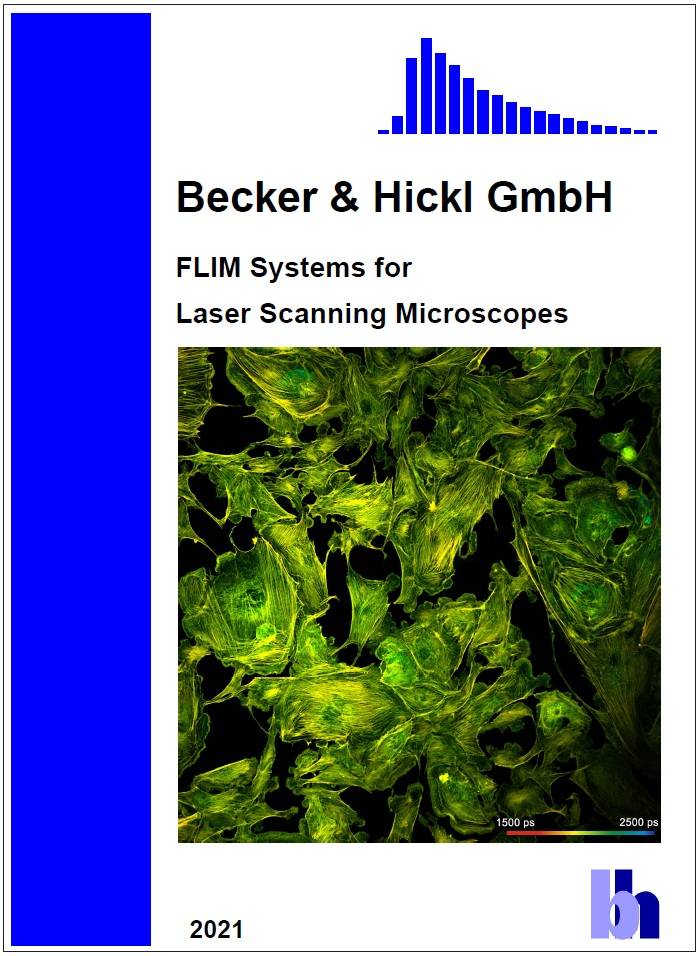
bh FLIM systems are unsurpassed in time
resolution. With their fast detectors and negligible timing jitter of the
electronics, they accurately record fluorescence-decay components which previously
were unknown to even exist. Moreover, the systems feature unbelievably high
timing stability. The time resolution does not degrade over extended
acquisition times, see Fig. 1. Extremely weak signals or signals from extremely
fragile samples can therefore be recorded successfully. The high stability in
combination with sophisticated data analysis makes it unnecessary to
re-calibrate the system by repeated recording of the instrument-response
function (IRF). This is a significant advantage for practical use.
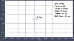

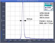
Fig. 1: Left to right: Electrical IRF of a bh FLIM system, timing
stability over 100 seconds, IRF with a HPM-100-06 detector
In addition, the bh FLIM systems feature
near-ideal photon efficiency and minimum acquisition time to reach a given
accuracy for a given photon rate. The pixels of the recorded FLIM images
contain precision fluorescence decay curves in a large number of time channels,
allowing the user to derive multi-exponential decay parameters from the data.
The most intriguing feature is the multi-dimensional nature of the recording
process. bh FLIM systems are able to record at several excitation wavelengths
simultaneously, record dynamic processes in live samples down to the
millisecond range, record FLIM and PLIM simultaneously, or record
multi-spectral FLIM images. With these capabilities, bh FLIM systems are able
to observe several parameters of biological system simultaneously, and in their
mutual dependence.
Principle
The FLIM systems are based on bh's
multi-dimensional time-correlated single photon counting (TCSPC) process in
combination with confocal or multiphoton scanning by a high-frequency pulsed
laser beam. Each photon is characterised by its time in the laser pulse period
and the coordinates of the laser spot in the scanning area in the moment of its
detection. The recording process builds up a photon distribution over these
parameters [24]. The result is an array of pixels, each containing a full
fluorescence decay curve in a large number of time channels [27, 33, 34].
Fig. 2: bh's
multi-dimensional TCSPC FLIM process probes the sample by randomly emitted
photons
The principle shown in Fig. 2 works at even
the fastest scan rates available in laser scanning microscopes. They combine
near-ideal photon efficiency, excellent time resolution, excellent timing
stability, fast recording speed, multi-wavelength capability, and resolution of
multi-exponential decay functions into their components with optical sectioning
capability and suppression of lateral scattering [30, 33]. The principle can be
extended to record at several laser wavelengths simultaneously, record
multi-wavelength FLIM images, record fast physiological effects in the sample,
record spatial mosaics and Z stacks of FLIM images, or to simultaneously record
fluorescence and phosphorescence lifetime images.
Most of the bh FLIM systems contain two or
more of the recording channels shown in Fig. 2. By using parallel channels,
high throughput is achieved, and crosstalk between the channels is avoided. The
channels of a bh FLIM system can be operated with laser multiplexing to record
signals excited by different laser wavelength quasi-simultaneously. The
principle is shown in Fig. 3.
Fig. 3:
Dual-channel TCSPC-FLIM system with laser multiplexing
Two lasers of different wavelength are
multiplexed at high rate. The TCSPC/FLIM modules receive a signal that
indicates which of the lasers was active in the moment when a photon was
detected. The TCSPC modules are thus able to build up separate photon
distributions for the photons excited by different lasers. With two lasers and
two TCSPC modules images for four combination of excitation and emission
wavelength are recorded simultaneously.
The principle shown in Fig. 2 can also be extended to simultaneously
detect in 16 wavelength channels. The optical spectrum of the fluorescence
light is spread over an array of 16 detector channels. The TCSPC system
determines the detection times, the channel numbers in the detector array, and
the position, x, and y, of the laser spot for the individual photons. These
pieces of information are used to build up a photon distribution over the time
of the photons in the fluorescence decay, the wavelength, and the coordinates
of the image. The principle of multi-wavelength FLIM is
shown in Fig. 4.
Fig. 4: Principle of Multi-Wavelength TCSPC FLIM
As for single-wavelength FLIM, the result of the recording process
is an array of pixels. However, the pixels now contain several decay curves for
different wavelength. Each decay curve contains a large number of time
channels; the time channels contain photon numbers for consecutive times after
the excitation pulse.
All bh FLIM systems are using 64-bit data
acquisition software [34]. As a result, images with extremely high spatial and
temporal resolution can be recorded. Images can be large as
2048 x 2048 pixels with 256 time channels per pixel, or
1024 x 1024 pixels with 1024 time channels. Such images cover the
full field of view of even the best microscope lenses at diffraction-limited
resolution. Multiwavelength FLIM is possible with 16 wavelength intervals and
up to 512 x 512 pixels and 256 time channels.
Data Acquisition Hardware
The bh FLIM system contain one or several
(usually two) TCSPC FLIM modules, a detector controller, and, if the bh DCS-120
scan head is used, a scan controller module. Different TCSPC modules, a
detector controller module, and a scanner control module [24] are shown in Fig.
5.
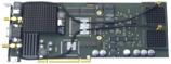
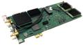
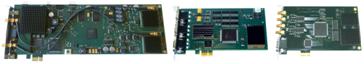
Fig. 5: Left to right: SPC-150 NX, SPC-180 NX, SPC-160 TCSPC
Modules, DCC-100 detector controller, GVD-120 scan controller
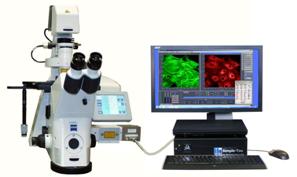
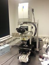
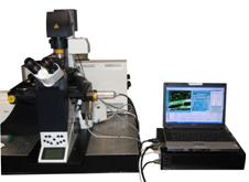
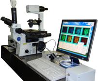
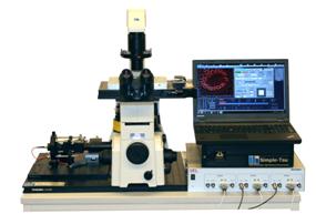
The modules can be operated inside a PC, or
in an extension box connected to a PC or a laptop computer, see Fig. 6.
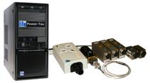
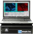
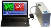
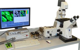
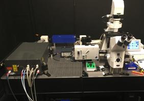
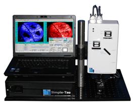
Fig. 6: Left: PC-based FLIM system, shown with DCS-120 scan head, BDL-SMC
picosecond diode laser, and HPM-100 hybrid detectors. Middle: Simple-Tau 152
dual-channel FLIM system. Right: Simple-Tau II system.
Excitation Sources
bh FLIM systems are compatible with almost
any high-frequency pulsed excitation source. One-photon FLIM systems usually
use picosecond diode lasers, see Fig. 7.
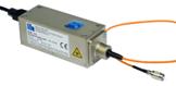
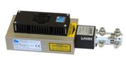
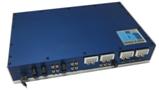
Fig. 7: bh picosecond diode lasers. Left to right: BDS-SM laser with fibre
output, BDS-SM laser with fibre coupler, LHB-104 'Laser Hub' with four lasers
emitting through one single-mode fibre.
FLIM upgrades for multiphoton microscopes of
external manufacturers normally use Titanium-Sapphire lasers which are
integrated in these systems. The DCS-MP multiphoton system of bh is available
both with a Titanium-Sapphire laser and with a single- or dual-wavelength
femtosecond fibre laser [20, 34].
Detectors
Most bh FLIM systems are using the bh
HPM-100 hybrid detectors [29]. The
advantage of these detectors is that they have a fast and clean TCSPC response
(IRF), and that they have no afterpulsing. The fast IRF and the absence of
afterpulsing background have the effect that FLIM data analysis works close to
the theoretical limit of photon efficiency [25]. Two versions of the HPM-100
are used for FLIM. The HPM-100-40 is used in applications which require highest
sensitivity, the HPM-100-06 in applications which require highest time
resolution. Detectors and detector assemblies are available with adapters for a
wide variety of microscopes. The detectors for confocal ports of one-photon
microscopes are compatible with those for NDD ports of multiphoton microscopes.


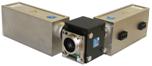
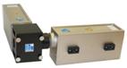
Fig.
8: HPM-100 hybrid detector and detector assemblies with different optical
adapters
In addition to the HPMs, bh guarantee that
the TCSPC systems work with any other single-photon detector as well. The
systems work with single-photon avalanche diodes (SPADs), with InGaAs SPADs [3],
with conventional PMTs [4],
with MCP PMTs [26], and even with superconducting NbN detectors [7, 38]. Please see [34] for details.
Data Acquisition Software
The bh FLIM systems use bh SPCM data
acquisition software [34].
Since 2013 the SPCM software is available in a 64-bit version. SPCM 64 bit
exploits the full capability of Windows 64 bit, resulting in faster data
processing, capability of recording images with extremely large pixel numbers,
and availability of additional multi-dimensional FLIM modes.
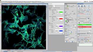
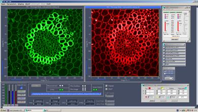
The main panel of the SPCM data acquisition
software is configurable by the user. Four configurations for FLIM systems are
shown in Fig. 9. During the acquisition the SPCM software displays intermediate
results in predefined intervals, usually every few seconds. The acquisition can
be stopped after a defined acquisition time or by a user commend when the
desired signal-to-noise ratio has been reached. Frequently used operation modes
and user interface configurations are selected from a panel of predefined
setups.
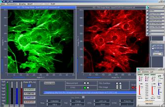
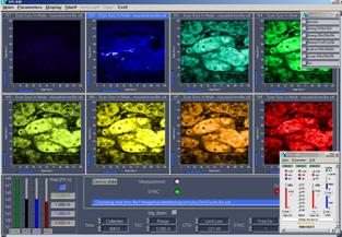
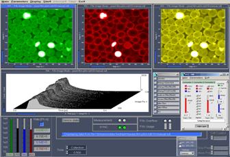
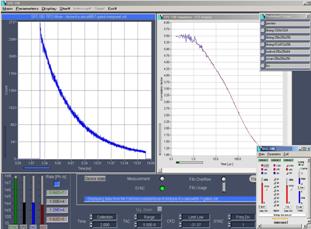
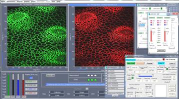
Fig. 9: SPCM software panel. Top left to bottom right: FLIM with two
detector channels, multi-spectral FLIM, combined fluorescence / phosphorescence
lifetime imaging (FLIM/PLIM), fluorescence correlation (FCS).
FLIM Data Analysis
All bh FLIM
systems use bh SPCImage NG data analysis software. SPCImage NG runs a
de-convolution on the decay data in the pixels of FLIM data. It uses single,
double, or triple-exponential decay analysis to produce pseudo-colour images of
lifetimes, amplitudes, or intensities of decay components, or of ratios of
these parameters. An incomplete decay model is available to determine long
fluorescence lifetimes within the short pulse period of the Ti:Sa laser of a
multiphoton system. Moreover, SPCImage NG avoids troublesome recording of an
instrument response function (IRF) by extracting the IRF from the FLIM data
themselves. SPCImage NG uses an MLE algorithm in combination with GPU
processing. This reduces the data processing time from formerly tens of minutes
to a few seconds.
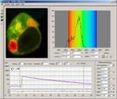
The main panel
of the SPCImage data analysis is shown in Fig. 10. It shows a lifetime image calculated
from the decay data in the pixels (left), a lifetime distribution over the
pixels of a region of interest (upper middle), and the fluorescence decay curve
in a selected spot of the image (lower right). The basic model parameters (one,
two or three exponential components) are selected in the upper right. Please
see [1, 2] or [34] for a detailed description of FLIM data analysis.
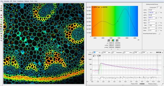
Fig. 10: Main panel of the SPCImage data
analysis
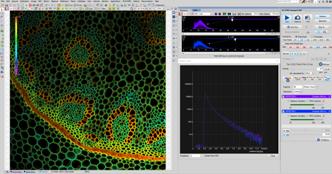
Since 2018 SPCImage combines time-domain
analysis with a phasor plot [40].
Pixels with different decay profiles are represented as different clusters of
phasors in the phasor plot. Cells of different lifetimes therefore form
separate clusters of phasors marked with different colours in the phasor plot,
see Fig. 11, right.
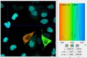
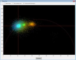
Fig. 11: SPCIMage, lifetime image and Phasor plot. The clusters in the
phasor plot represent pixels of different lifetime in the lifetime image.
Recorded by bh Simple-Tau 152 FLIM system with Zeiss LSM 880.
Pixels with similar phasor signature can be
combined, and the combined data be used for high-accuracy multi-exponential
decay analysis. Please see chapters SPCImage NG Data Analysis in [1, 13, 34]
and SPCImage NG Overview brochure [21].
FLIM Functions in Brief
Easy Change Between Instrument Configurations
Frequently used instrument configurations
are stored in a Predefined Setup panel. Changing between the different
configurations and user interfaces is just a matter of a single mouse click,
see Fig. 12.
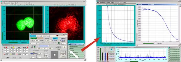
Fig. 12: Changing between different instrument configurations: The software
switches from a FLIM configuration into an FCS configuration by a simple mouse
click
Interactive Scan Control
Any change in the scan area of the
microscope immediately becomes effective in the recorded images.
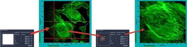
Fig. 13: Interactive scanner control for external microscope software.
Example for Zeiss LSM 780/880.
For systems using the GVD-120 (such as the
bh DCS 120 system) the control of the scanner is integrated in the SPCM data
acquisition software. The zoom factor and the position of the scan area can be
adjusted via the scanner control panel or via the cursors of the display window.
Changes in the scan parameters are executed online, without stopping the scan.
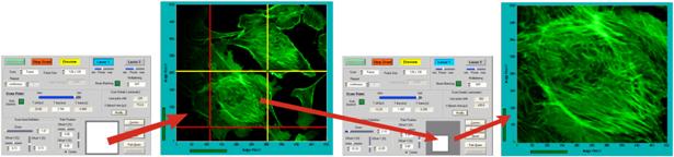
Fig. 14:
Interactive scanner control for systems using the bh GVD-120 scan controller
module
Fast preview function
When FLIM is applied to live samples the
time and the sample exposure needed for positioning, focusing, laser power
adjustment, and selection of the scan region has to minimised. Therefore, the bh
FLIM systems have a fast preview function. The preview function displays images
in intervals of 1 second and faster. Both intensity and lifetime images can be
displayed. The preview function can be combined with fast online-FLIM display,
please see Fig. 33, page 19.
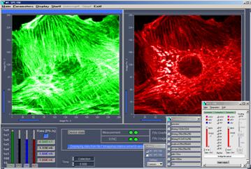
Fig. 15: SPCM software in fast preview mode. 1 image per second, two
parallel FLIM channels recording in separate wavelength intervals.
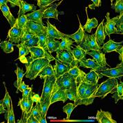
Two fully parallel TCSPC FLIM Channels
Standard bh FLIM systems record in two
wavelength intervals simultaneously. The signals are detected by separate
detectors and processed by separate TCSPC modules [34]. There is no intensity
or lifetime crosstalk. Even if one channel overloads the other channel is still
able to produce correct data. More parallel channels can be added if necessary,
please see [34].
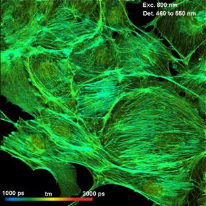
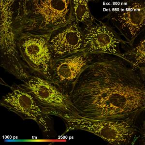
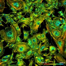
Fig. 16: Dual-channel detection. BPAE
cells stained with Alexa 488 phalloidin and Mito Tracker Red. Left: 460 nm
to 550 nm. Right: 550 nm to 650 nm.
Online FLIM Display
Online FLIM display is available for all
versions of the bh FLIM systems. The function is based in first-moment
calculation. It delivers a near-ideal signal-to-noise ratio for the
single-exponential lifetime of the decay data, see [34]. An example of the SPCM
main panel for dual-channel lifetime display is shown in Fig. 17.
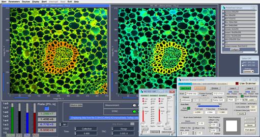
Fig. 17: SPCM main panel for online-lifetime display, dual channel system
Ultra-High Time Resolution: FLIM with <20ps IRF width
In combination
with the ultra-fast HPM-100-06 and -07 detectors, bh multiphoton FLIM systems
system achieve an instrument response function (IRF) of less than 20 ps FWHM [8]. The fast response greatly improves the accuracy at which fast decay
components can be extracted from a multi-exponential decay. Applications are
mainly in the field of metabolic imaging. In the past few years the field has
been rapidly expanding [34]. Metabolic FLIM requires separation of the decay
components bound and unbound NADH. Typical NADH FLIM images of the
amplitude-weighted lifetime and of the amplitudes and lifetimes of the fast and
slow decay component are shown in Fig. 18
and Fig. 19. Please see [10] for details. Clinical applications are
described in [37, 43].
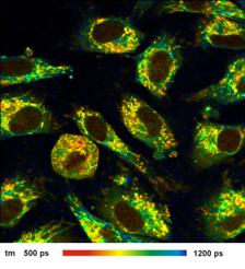
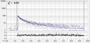
Fig. 18: NADH Lifetime
image, amplitude-weighted lifetime of double-exponential fit. Right: Decay
curve in selected spot, 9x9 pixel area. FLIM data format 512x512 pixels, 1024
time channels. Time-channel width 10 ps.
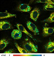
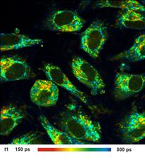
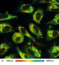
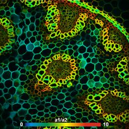
Fig. 19: Left to right:
Images of the amplitude ratio, a1/a2 (unbound/bound ratio), and of the fast
(t1, unbound NADH) and the slow decay component (t2, bound NADH). FLIM data
format 512x512 pixels, 1024 time channels. Time-channel width 10ps.
The high time resolution of the bh
multiphoton FLIM systems [20] makes fluorescence-decay components visible which
have never been detected before. Fig. 20 shows FLIM data of mushroom spores, which
show a dominating decay component of 12 ps lifetime [22]. In Pollen
grains, the DCS-MP system detects a component with 10 ps lifetime [23],
see Fig. 21. In principle, ultra-fast decay components are detectable also with
other multiphoton microscopes, if the bh SPC-150 NX or SPC-180 NX
TCSPC modules and HPM-100-06 detectors are used.
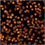
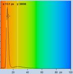
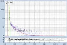
Fig. 20: 2p
FLIM of Mushroom Spores. The fast component has a lifetime of t1 = 12 ps
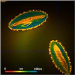
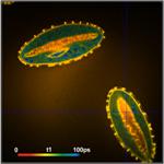
Fig. 21: 2p
FLIM of Pollen Grains. The fast component has a lifetime of t1 = 10 ps
Multiphoton NDD FLIM: Clear Images from Deep Tissue Layers
bh FLIM systems for multiphoton microscopes
are compatible with non-descanned detection (NDD). With non-descanned
detection, fluorescence photons scattered on the way out of the sample are
detected efficiently and assigned to the correct pixels of the image. The
result is that bright and clear images are obtained from deep tissue layers. An
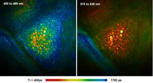
example is shown in Fig. 22.
Fig. 22: Two-photon FLIM of pig skin. LSM 710 NLO, HPM‑100‑40,
NDD. Left: Wavelength channel <480nm, colour shows percentage of SHG.
Right: Wavelength channel >480nm, colour shows amplitude-weighted mean
lifetime.
Metabolic FLIM by Multiplexed
Excitation
The bh DCS-120
Confocal Scanning FLIM System detects changes in the metabolic state of live
cells [19]. Information on the metabolic state is derived from the fluorescence
decay functions of NAD(P)H and FAD. Two ps diode lasers, with wavelengths of
375nm and 405 nm, are multiplexed to alternatingly excite NAD(P)H and FAD. One
FLIM channel of the DCS system detects in the emission band of NAD(P)H, the
other in the emission band of FAD. A result is shown in Fig. 23.

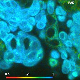
Fig. 23: a1
images (amplitude of fast component) of NAD(P)H (left) and of FAD (right)
The FLIM data are
processed by SPCImage data analysis software. For both channels, the data
analysis delivers images of the amplitude-weighted lifetime, tm, the component
lifetimes, t1 and t2, the amplitudes of the components, a1 and a2, and the
amplitude ratio, a1/a2. Moreover, it delivers the fluorescence-lifetime redox
ratio (FLIRR), a2nadh/a1fad. For
theoretical background and technical details please see [19, 34]. Clinical
applications are described in [37, 43]. Metabolic FLIM can be combined with pO2
measurement by simultaneous FLIM / PLIM. Please see page 24 of this brochure.
Megapixel FLIM Images
With 64 bit SPCM software pixel numbers can
be increased to 2048 x 2048 pixels, with a temporal resolution of 256
time channels. Two such images can be recorded simultaneously in different
wavelength channels.
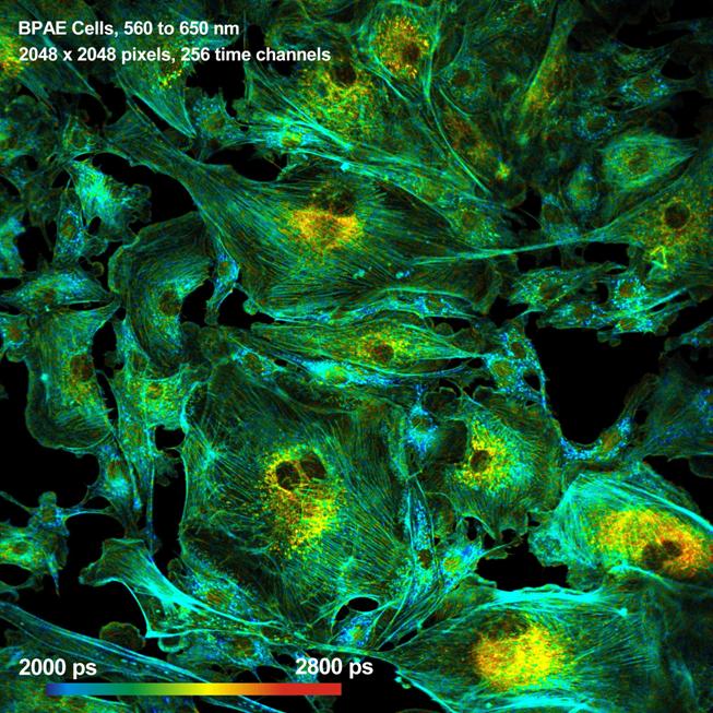
Fig. 24: BPAE cells, recorded with a
spatial resolution of 2048 x 2048 pixels. 256 time channels per
pixel.
With its capability to record large images
the bh FLIM technique is also able to record spatial mosaic FLIM data or mosaics
of images over time, depth in the sample, or emission wavelength. Please see Fig.
25, Fig. 29, Fig. 30, Fig. 36, and Fig. 37.
Multi-Spectral FLIM
bh FLIM systems are able to record
simultaneously in 16 wavelength channels. The images are recorded by an
extended multi-dimensional TCSPC process which uses the wavelength of the
photons as a coordinate of the photon distribution [28, 34]. An example is shown in Fig. 25.
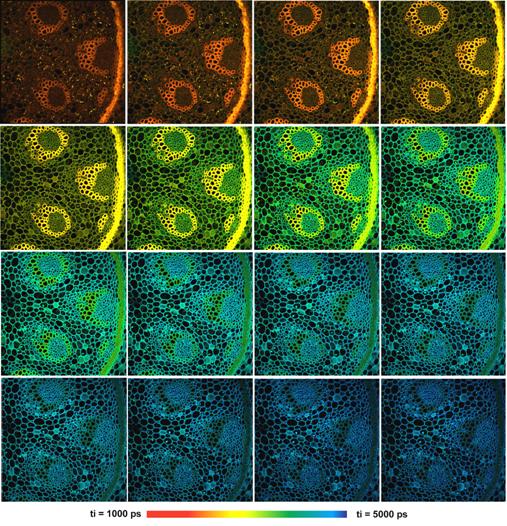
Fig. 25: Multi-wavelength FLIM, 16
images with 512 x 512 pixels and 256 time channels were recorded
simultaneously. bh DCS‑120 confocal scanner, bh MW-FLIM GaAsP 16-channel
detector, Zeiss Axio Observer microscope.
There is no time gating, no wavelength
scanning and, consequently, no loss of photons in this process. The system thus
reaches near-ideal recording efficiency. Moreover, dynamic effects in the
sample or photobleaching do not cause distortions in the spectra or decay
functions. The individual images in the 16 wavelength channels are recorded at
a resolution of up to 512x512 pixels and 256 time channels.
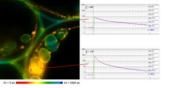
Fig. 26 and Fig. 27 demonstrate the true
resolution of the data. Images from two wavelength channels, 502 nm and
565 nm, were selected form the data shown Fig. 25, and displayed at larger
scale and with individually adjusted lifetime ranges. With 512x512 pixels and
256 time channels, the spatial and temporal resolution of the individual images
is comparable with that normally used for single-wavelength FLIM.
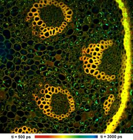
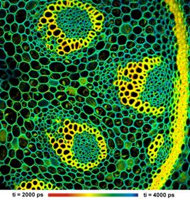
Fig. 26: Two images from the array shown
in Fig. 25, displayed in larger scale and with individually adjusted lifetime
range. The images have 512 x 512 pixels and 256 time channels.
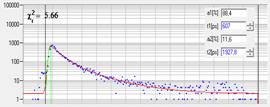
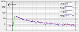
Fig. 27: Decay curves at selected pixel position in the images shown above.
Blue dots: Photon numbers in the time channels. Red curve: Fit with a
double-exponential model.
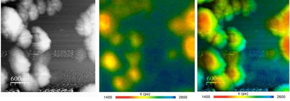
Multiphoton Multispectral NDD FLIM
bhs MW FLIM is the worlds first
simultaneously detecting multiphoton multispectral NDD FLIM system [28]. It uses
a special optical interface that connects the NDD ports of multiphoton
microscopes to the input slit of the detector [1, 2, 34]. A typical result is
shown in Fig. 28.
Fig. 28: Multiphoton Multispectral NDD FLIM. Plant tissue, lifetime images
and decay curves in selected pixels and wavelength channels. Recorded with LSM 710
NLO and bh MW FLIM detector
Mosaic FLIM is based on bhs Megapixel
FLIM technology introduced in 2014. Mosaic FLIM records a large number of
images into a single FLIM data array [34]. The individual images within this
array can be for different displacement of the sample (lateral mosaic),
different depth within the sample (z-stack mosaic), of for different times
after a stimulation of the sample (temporal mosaic). Lateral mosaic FLIM
combines favourably with the Tile Imaging capability of the Zeiss LSM 710/780/880
and similar procedures in other microscopes. An example is shown in Fig. 29.
The complete data array has 2048 x 2048 pixels, and 256 time channels
per pixel. Compared to a similar image taken through a low-magnification lens
the advantage of mosaic FLIM is that a lens of higher numerical aperture can be
used, resulting in higher detection efficiency and higher spatial resolution.
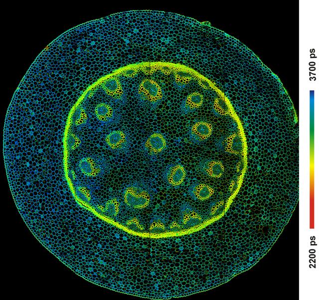
Fig. 29: Mosaic FLIM of a Convallaria sample. The mosaic has 4x4 elements,
each element has 512x512 pixels with 256 time channels. The complete mosaic has
2048 x 2048 pixels, each pixel holding 256 time channels. Zeiss
LSM 710 with bh Simple-Tau 150 FLIM system. Total sample size covered
by the mosaic 2.5 x 2.5 mm.
The Mosaic FLIM function can be used to
record Z Stacks of FLIM images. As the microscope scans consecutive image
planes the FLIM system records the data into consecutive elements of a FLIM
mosaic. The advantage over the traditional record-and-save procedure (page 18)
is that no time has to be reserved for save operations, and that the entire
array can be analysed in a single data analysis run.
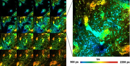
Fig. 30: FLIM Z-stack, recorded by Mosaic FLIM. Pig skin stained with DTTC.
16 planes, 0 to 60 um from top of tissue. Each element of the FLIM mosaic
has 512x512 pixels and 256 time channels per pixel. Plane 8 is shown magnified
on the right. LSM 7 OPO system, HPM-100-50 GaAs hybrid detector.
The bh FLIM systems are able to record Z
stacks of FLIM images [1, 34] also by a conventional record-and-save procedure.
For each Z plane, a FLIM image is scanned and acquired for a specific
collection time. Then the data are saved in a file, the microscope steps to
the next plane, and the next image is acquired. The procedure continues for a
specified number of Z planes. A Z stack of autofluorescence images taken at a water
flee is shown in Fig. 31.
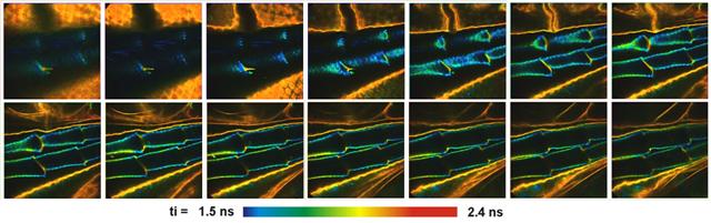
Fig. 31: Z stack recording, part of a water flee, autofluorescence. Images
256x256 pixels, 256 time channels.
Another way of recording Z stacks is by
Mosaic FLIM. In that case, the images of the individual planes are recorded in
subsequent elements of a FLIM data mosaic. Please see Z Stack Mosaic FLIM,
page 18.
Time-Series FLIM by Record-and-Save Procedure
Time-series FLIM is available for all
system versions, and all detectors [1, 2, 34]. Time series as fast as 2 images
per second can be obtained. A time series taken at a moss leaf is shown in Fig.
32. Time-series FLIM at higher speed can be performed by temporal mosaic FLIM,
see Fig. 36 and Fig. 37. Time-series FLIM can be combined with online-FLIM
display, please see section above.
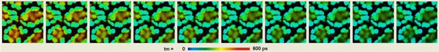
Fig. 32:
Time-series FLIM, 1 image per second. Chloroplasts in a leaf, the fluorescence
lifetime of the chlorophyll decreases with the time of exposure.
Fast Online FLIM
The bh TCSPC/FLIM systems record and
display fluorescence lifetime images at a rate of up to 10 images per second [11,
14]. The function is normally used to select interesting cells within a larger
sample for subsequent high-accuracy FLIM acquisition. In FLIM experiments with
longer acquisition time it helps the user evaluate the signal-to-noise ratio of
the data and decide whether enough photons have been recorded to reveal the
expected lifetime effects in the sample.
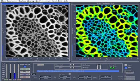
Fig. 33: Fast online FLIM. Intensity
image (left) and lifetime image (right). Images 128 x 128 pixels,
recorded at a speed of 5 images per second.
The bh FASTAC Fast-Acquisition FLIM System
The bh Fast-Acquisition FLIM system uses
four parallel TCSPC channels and a device that distributes the photon pulses of
a single detector into the four recording channels [15, 16, 17]. The system
features an electrical IRF width of less than 7 ps (FWHM), and a time
channel width down to 820 fs. The optical time resolution with an
HPM-100-06 or -07 hybrid detector is shorter than 25 ps (FWHM). The system
is virtually free of pile-up effects. FLIM data can be recorded at acquisition
times down to the fastest frame times of the commonly used galvanometer
scanners. The data are recorded with the TCSPC-typical number of time-channels
of up to 4096, and with pixel numbers from 128 x 128 to 2048 x 2048
pixels. The system is therefore equally suitable for fast FLIM and precision
FLIM applications.
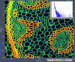
Fig. 34:
FASTAC FLIM. Left: 256x256 pixels, acquisition time 0.5 s. Insert: Decay data
in 10x10 pixel area. Right: IRF
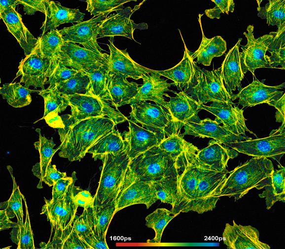
Fig. 35: High-accuracy FLIM image,
recorded in 10 seconds. 1024 x 1024 pixels, 1025 time channels.
FASTAC FLIM system with Zeiss LSM 880 NLO multiphoton microscope.
Mosaic FLIM can be used to record FLIM time
series. The recording principle is the same as for lateral mosaic FLIM, except
for the fact that the sample is not moved between the individual recordings.
The result is thus a mosaic of FLIM images for consecutive times after the
start of an experiment. An example is shown in Fig. 36.

Fig. 36: Time series acquired by mosaic
FLIM. Recorded at a speed of 1 mosaic element per second. 64 elements, each
element 128 x 128 pixels, 256 time channels, double-exponential fit
of decay data. Sequence starts at upper left. Moss leaf, lifetime changes by
non-photochemical chlorophyll transient.
Faster than Fast FLIM: Temporal Mosaic FLIM with Triggered
Accumulation
The advantage of Mosaic FLIM is that no
time has to be reserved for save operations between the recording of the
individual images. A Mosaic-FLIM time series can therefore be made very fast.
The most important advantage is, however, that temporal Mosaic FLIM data can be
accumulated. A lifetime change in the sample is stimulated periodically, and a
mosaic recording sequence started for each stimulation. Because the entire
photon distribution is kept in the memory the photons from the subsequent runs
are automatically accumulated. The result is that the signal-to-noise ratio no
longer depends on the speed of the series. The only speed limitation is the
minimum frame time of the scanner. For many laser scanning microscopes frame
times of less than 50 milliseconds can be achieved [39]. This brings the
transient-time resolution down to the range where physiological effects in live
samples occur. A typical application is the recording of Ca2+
transients in neurons. An example is shown in Fig. 37.
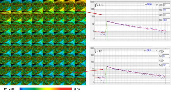
Fig. 37: Temporal mosaic FLIM of the Ca2+
transient in cultured neurons after stimulation with an electrical signal. The
time per mosaic element is 38 milliseconds, the entire mosaic covers 2.43
seconds. Experiment time runs from upper left to lower right. Photons were
accumulated over 100 stimulation periods. Zeiss LSM 7 MP multiphoton microscope
and bh SPC‑150 TCSPC module. Data courtesy of Inna Slutsky and Samuel
Frere, Tel Aviv University, Sackler Faculty of Medicine.
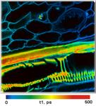
FLITS: Fluorescence Lifetime-Transient Scanning
FLITS records transient effects in the
fluorescence lifetime of a sample along a one-dimensional scan. The technique
is based on building up a photon distribution over the distance along the scan,
the arrival times of the photons after the excitation pulses, and the experiment
time after a stimulation of the sample. The maximum resolution at which
lifetime changes can be recorded is given by the line scan time. With
repetitive stimulation and triggered accumulation transient lifetime effects
can be resolved at a resolution of about one millisecond [31].
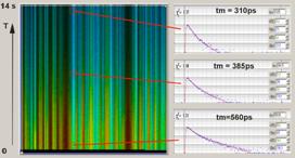
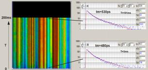
Fig. 38: FLITS of chloroplasts in a grass
blade, change of fluorescence lifetime after start of illumination. Left:
Non-photochemical transient, transient resolution 60 ms. Right:
Photochemical transient. Triggered accumulation, transient resolution
1 ms.
Excitation Wavelength Multiplexing
By multiplexing several ps diode lasers
images can be obtained quasi-simultaneously for different excitation wavelength
[34]. With the two detection channels of the bh systems, images for three or
four combinations of excitation and emission wavelength are obtained. An example
is shown in Fig. 39.
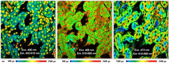
Fig. 39: Excitation wavelength
multiplexing, 405 nm and 473 nm. Detection wavelength 432 nm to
510 nm and 510 nm to 550 nm. Mouse kidney section, stained with
Alexa 488 WGA, Alexa 568 phalloidin, and DAPI.
Near-Infrared FLIM
Scattering coefficients in biological
tissue in the near-infrared region are lower than in the visible. Therefore,
FLIM with near-infrared dyes is a second way to obtain images from deep layers
of biological tissues. Different than for multiphoton FLIM, where only the
excitation is in the NIR, both the excitation and the emission are in the near
infrared. Therefore, deep-tissue imaging is possible even with one-photon
excitation and confocal detection. Moreover, many near-infrared dyes display
large lifetime variations with the local molecular environment and are thus
potential molecular markers. Near-infrared FLIM can be performed by one-photon
excitation with ps diode lasers, by one-photon excitation with Ti:Sapphire
lasers, or two-photon excitation by an OPO [5, 32]. Please see Fig. 40, Fig. 41 and Fig.
42.
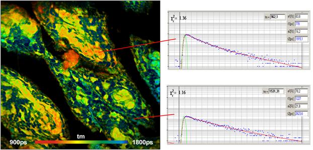
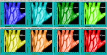
Fig. 40: Near-Infrared FLIM with picosecond diode laser, bh DCS-120 system.
Pig skin sample stained with 3,3-diethylthiatricarbocyanine, detection
wavelength from 780 nm to 900 nm.
Fig. 41: Pig skin samples stained with 3,3-diethylthiatricarbocyanine.
Zeiss LSM 780 NLO system, one-photon excitation by Ti:Sa laser at 780nm,
confocal detection at 800nm to 900nm
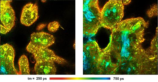
Fig. 42: Pig skin stained with
Indocyanin Green. Zeiss LSM 780 OPO system, two-photon excitation at
1200 nm, non-descanned detection, 780 to 850 nm. Depth from top of
tissue 10 µm (left) and 40 µm (right).
Phosphorescence and fluorescence lifetime
images are recorded simultaneously by bhs proprietary FLIM/PLIM technique. The
technique is based on modulating a ps diode laser synchronously with the pixel
clock of the scanner. FLIM is recorded during the On time, PLIM during the
Off time of the laser [9, 34,
35, 44]. The SPCM software delivers separate images for the fluorescence and
the phosphorescence which are then analysed with SPCImage FLIM/PLIM analysis
software.
Currently, there is increasing interest in
PLIM for background-free recording and, especially, for oxygen sensing. In
these applications, the bh technique delivers a far better sensitivity than
PLIM techniques based on single-pulse excitation. The real advantage of the bh FLIM/PLIM
technique is, however, that FLIM and PLIM are obtained simultaneously.
It is thus possible to record metabolic information via FLIM of the NADH and
FAD fluorescence, and simultaneously map the oxygen concentration via PLIM [41,
42]. The number of publications in this area is literally exploding, please see
FLIM/PLIM chapters in [1], [2] or [34]. An example is shown in Fig. 43.
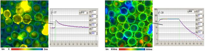
Fig. 43: Yeast cells stained with (2,2-bipyridyl) dichlororuthenium (II)
hexahydrate. FLIM and PLIM image, decay curves in selected spots.
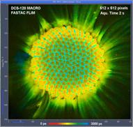
FLIM of Macroscopic Objects
With the bh DCS-120 MACRO version objects
as large as 15 mm can be scanned [2]. Image obtained with the DCS-120
MACRO is shown in Fig. 44 and Fig. 45.
Fig. 44: FLIM of a macroscopic object. Resolution 2048 x2048 pixels, 256
time channels. Left: Original image. Right: digital zoon into recorded FLIM
image, showing the excellent resolution of the data.
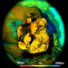
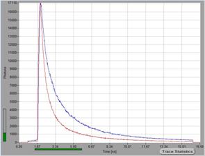
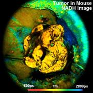
Fig. 45:
Tumor in a live mouse. NADH FLIM image (left) and decay curves inside and
outside tumor (right).
Scanning of Well Plates
With an
optional motor stage, both the DCS-120 and the DCS MACRO system can be used to
scan well plates. An example is shown in Fig. 46.
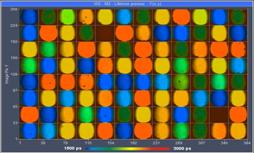
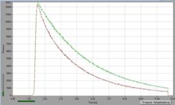
Fig. 46: Well
plate scanned with DCS-120 MACRO. Lifetime image and decay functions in wells 4
and 5, lower row.
STED FLIM
TCSPC FLIM can be
combined with STED [34]. The combination of a STED microscope of Abberior
Instruments (Göttingen, Germany) with the bh Simple-Tau 150/154 TCSPC FLIM
system records FLIM data at a spatial resolution of better than 40 nm. The
image format can be as large as 2048 x 2048 pixels, with 256 time
channels per pixel. An image area of 40 x 40 micrometers can
thus be covered with 20 nm pixel size, fully satisfying the Nyquist
criterion. With smaller numbers of time channels even larger pixel numbers are
possible. The system especially benefits from Windows 64 bit technology used
both in the Abberior and in the bh data acquisition software, from the combined
processing power of two parallel system computers, and the high data throughput
of up to four parallel TCSPC FLIM channels. The system achieves peak count
rates in excess of 5 MHz per FLIM channel, resulting in unprecedented
signal-to-noise ratio and short acquisition time.
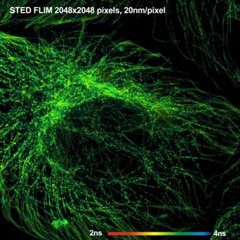
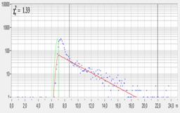
Fig. 47: STED FLIM with Abberior Instruments
STED microscope. 2048 x 2048 pixels. Single cell, stained with tubulin-binding
dye, recorded at a resolution of 20 nm per pixel. Decay curve in selected
pixel shown on the right. The initial peak is undepleted fluorescence. It is
gated off in the intensity data of image shown on the left.
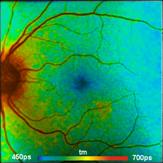
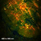
Clinical FLIM
Clinical FLIM applications use the fact
that pathological processes induce changes in the molecular environment or in
the conformation of endogenous fluorophores. These, in turn, cause detectable
changes in the fluorescence decay profiles. bh FLIM has been introduced into clinical
instruments for ophthalmology and dermatology. Developments for other
applications are in progress. Please see [33] or [34] for an overview and for
technical details. The first clinical instruments are on the market. FLIM
images recorded with the FLIO Fluorescence Lifetime Ophthalmoscope of
Heidelberg Engineering and with the MPT Flex multiphoton skin tomography system
of Jenlab are shown in Fig. 48.
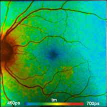

Fig. 48: Left: FLIM of a human retina, recorded in vivo with Heidelberg
Engineering FLIO ophthalmoscope. Right: Multiphoton FLIM of human skin, recorded
in vivo with Jenlab MPT FLEX multiphoton tomography system.
FCS
The bh GaAsP
hybrid detectors of the bh FLIM systems deliver highly efficient FCS [1, 29, 34]. Because the detectors are free
of afterpulsing there is no afterpulsing peak in the autocorrelation data. Thus,
accurate diffusion times and molecule parameters are obtained from a single
detector. Compared to cross-correlation of split signals, correlation of
single-detector signals yields a four-fold increase in correlation efficiency.
The result is a substantial improvement in the SNR of FCS recordings [29, 34].
FCS is be obtained both with confocal systems and with multiphoton NDD systems.
Gated FCS is obtained by hardware gating the photon times within the TCSPC
modules, FCCS by cross-correlating the signals of two TCSPC channels.
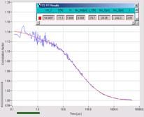
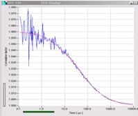
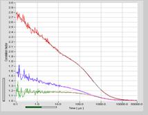
Fig. 49: FCS with bh TCSPC FLIM systems,
GaAsP hybrid detectors. Left to right: Confocal FCS with ps diode laser,
two-photon NDD FCS, cross correlation of photons recorded in different
detection channels.
bh FLIM Systems for
Various Microscopes
DCS-120 Confocal Scanning FLIM Systems
FLIM at image size up
to 2048 x 2048 pixels
Complete Confocal
Laser Scanning FLIM microscopes
FLIM upgrade for
existing conventional microscopes
Scanning by fast
galvanometer mirrors
Two fully parallel confocal
detection channels
One or two BDL-SMC or
BDL-SMN picosecond diode lasers
Laser wavelengths
375, 405, 440, 473, 488, 510, 640, 685, 785 nm
Wideband (WB)
version, compatible with tuneable lasers
Channel separation by
dichroic or polarising beamsplitters
Individually
selectable pinholes, individually selectable filters
bh HPM-100-40 GaAsP
hybrid detectors
Optional HPM-100-06
detectors for ultra-high time resolution
GaAs hybrid detectors
for NIR range
Optional 16-channel
multi-wavelength GaAsP detector module
Z-stack FLIM
acquisition with Zeiss Axio Observer Z1
Simultaneous FLIM / PLIM
Optional motor stage,
control integrated in instrument software
Spatial and temporal
mosaic FLIM
Ultra-fast recording
of time series
Metabolic FLIM
Capability
Fluorescence
lifetime-transient scanning (FLITS)
Version with FASTAC
FLIM available
Please see [2] for
details
DCS-120 MP Multiphoton FLIM Systems
Excitation by fs Ti:Sa
laser or fs fibre laser
Laser intensity and
wavelength control integrated in SPCM data acquisition software
PLIM laser modulation
by DCS-120 scan controller and AOM, control functions integrated in instrument
software
Clear Images from
deep tissue layers
Excellent spatial and
temporal resolution
Full field of view of
microscope lens scanned
Images up to 2048 x
2048 pixels
Two non-descanned
detection channels,
Two optional confocal
channels
bh HPM-100-40 GaAsP hybrid
detectors
Optional HPM-100-06
detectors for ultra-high time resolution
Optional 16-channel
multi-wavelength GaAsP detector module
Z-stack FLIM
acquisition with Zeiss Axio Observer Z1
Simultaneous FLIM /
PLIM
Optional motor stage,
control integrated in instrument software
Spatial and temporal
mosaic FLIM
Ultra-fast recording
of time series
Metabolic-FLIM
capability
Fluorescence
lifetime-transient scanning (FLITS)
FASTAC FLIM system
available
Please see [2] for
details
DCS-120 Macro System
FLIM of macroscopic
objects
Scan field up to
15 mm diameter
FLIM with up to 2048
x 2048 pixels
Scanning by fast
galvanometer mirrors
Two fully confocal
detection channels
One or two BDL-SMC or
BDL-SMN picosecond diode lasers
Laser wavelengths
375, 405, 440, 473, 488, 510, 640, 685, 785 nm
Tuneable excitation
by super-continuum laser with AOTF
One or two confocal
detection channels, parallel acquisition
Channel separation by
dichroic or polarising beamsplitters
Individually
selectable pinholes, individually selectable filters
bh HPM-100-40 GaAsP
hybrid detectors
Optional HPM-100-06
detectors for ultra-high time resolution
GaAs hybrid detectors
for NIR range
16-channel
multi-wavelength GaAsP detector module
Optional motor stage,
control integrated in instrument software
Simultaneous
fluorescence and phosphorescence lifetime imaging (PLIM)
Metabolic FLIM
capability
Spatial and temporal
mosaic FLIM
Ultra-fast recording
of time series
Fluorescence
lifetime-transient scanning (FLITS)
Wideband (WB)
version, compatible with tuneable lasers
FASTAC FLIM system
available
Please see [2] for
details
FLIM Systems for Zeiss LSM 710 / 780 / 880 / 980
Microscopes
LSM 710 / 780 / 880 / 980 NLO, LSM 7MP Multiphoton
Microscopes
LSM 710, LSM 780, LSM 880, LSM 980 Confocal Microscopes
FLIM with up to 2048
x 2048 pixels
Multiphoton FLIM,
PLIM, multispectral FLIM, FCS
Confocal FLIM, PLIM,
multispectral FLIM, FCS
FLIM with bh HPM
hybrid detectors or Zeiss BIG-2 detectors
Fast preview mode,
both for intensity and lifetime
Mosaic FLIM
Z Stack FLIM
Fast Time-series FLIM
Acquisition by 1, 2,
3 or 4 parallel TCSPC FLIM channels
Detection by bh
HPM-100-40 GaAsP hybrid detectors or Zeiss BIG 2 detector
Optional HPM-100-06
detectors for ultra-high time resolution
Simultaneous
fluorescence and phosphorescence lifetime imaging (PLIM)
Fluorescence
lifetime-transient scanning (FLITS)
Spatial and temporal
mosaic FLIM
Ultrafast time-series
recording by temporal mosaic FLIM function
Confocal NIR FLIM up
to 900 nm detection wavelength
Two-Photon OPO FLIM
up to 900nm detection wavelength
FASTAC FLIM system
available
Please see [1] for
details
Still available: FLIM Systems for Zeiss LSM 510 NLO
Multiphoton Microscopes
FLIM with up to 2048
x 2048 pixels
Multiphoton
excitation with non-descanned detection
Single-wavelength and
Dual-wavelength NDD FLIM
Multi-spectral NDD
FLIM
Fast preview mode
Mosaic FLIM
Z Stack FLIM
Fast time-series FLIM
HPM‑100‑40
hybrid detectors
One or two parallel
SPC‑150 TCSPC channels
Portable to LSM 710,
780, 880 microscopes
Software-Integrated FLIM for Nikon A1+ Confocals
Integrated in Nikons
NIS-Elements Instrument Software
Excitation by bh
BDS-SM ps diode lasers
Detection by bh
HPM-100-40 GaAsP hybrid detectors
Two fully parallel
SPC-150N TCSPC FLIM channels
Data analysis by bh
SPCImage
Fast acquisition,
high optical resolution, high efficiency, high time resolution
Please see [18] for
details
Non-descanned FLIM Systems for Nikon A1 MP Multiphoton
Microscopes
64-bit megapixel FLIM
technology
One FLIM channel or
two parallel FLIM channels
High-efficiency
PMH-100 hybrid detectors
Non-descanned
detection for deep-tissue imaging
Multi-spectral FLIM
with 16-channel GaAsP detector
ROI and Zoom
functions of A1 available
Works at any scan
rate
Megapixel FLIM
Fluorescence
lifetime-transient scanning (FLITS)
Ultra-fast time series
by temporal mosaic FLIM
FASTAC FLIM system
available
FLIM Systems for Sutter Instrument MOM Microscopes
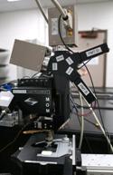
Up to four parallel
FLIM channels
Multiphoton
excitation by Ti:Sa laser
Non-descanned
detection for deep-tissue imaging
Overload protection
of FLIM detectors
Up to 1024 x 1024
pixels, 1024 time channels
High efficiency
Fast acquisition
SPCM Online FLIM
function available
Simultaneous FLIM /
PLIM
FASTAC FLIM system
available
Please see [12] for details.
Non-Descanned FLIM Systems for Leica SP5 MP, SP8 MP
Microscopes
Non-descanned
detection via Leica RLD port
1 detector coupled
directly to RLD port
2 detectors via
external beamsplitter
Simple-Tau 150 or 152
TCSPC systems
Acquisition in 1 or 2
parallel TCSPC FLIM channels
bh HPM‑100‑40
GaAsP hybrid detectors or Leica HYD detectors
Optional HPM-100-20
ultra-fast hybrid detectors
Multi-spectral FLIM
with 16-channel GaAsP detector
Works at any scan
rate of SP microscope
No nonlinearity by
Leica sinusoidal scan
Fast acquisition,
fast preview mode
Megapixel FLIM, 2048
x 2048 pixels
Fluorescence
lifetime-transient scanning (FLITS) and temporal mosaic FLIM available
Ultra-fast time
series by temporal mosaic FLIM
Simultaneous FLIM /
PLIM
FASTAC FLIM system
available
Please see [6] for
details.
Non-descanned FLIM Systems for Olympus Multiphoton
Microscopes
Multiphoton FV
systems with inverted microscopes
High efficiency by
non-descanned FLIM detection
Deep-tissue imaging
capability
HPM-100-40 GaAsP
hybrid detectors
Optional HPM-100-06
hybrid detectors for ultra-high time resolution
Optional 16-channel multi-spectral
GaAsP detector
Full overload
protection of FLIM detectors
ROI and Zoom
functions of available
Works at any scan
rate
Fluorescence
lifetime-transient scanning (FLITS) and temporal mosaic FLIM available
FASTAC FLIM system
available
PZ-FLIM-110 Stage-Scanning FLIM System
Sample scanning by
piezo scan stage
Excitation by BDL or
BDS series ps diode lasers
Confocal detection
HPM-100-40 GaAsP hybrid
detector
Optional HPM-100-06
hybrid detector for ultra-high time resolution
Optional PML-SPEC
GaAsP multi-spectral detector
Excellent contrast
and resolution
Fully controlled by
bh SPCM TCSPC/FLIM data acquisition software
Compact electronics,
integrated in bh Simple Tau system
Megapixel FLIM
technology - images up to 2048 x 2048 pixels
Lateral (x-y) an
vertical (z) scanning
Simultaneous FLIM /
PLIM
Please see [34] for
details.
FLIM for NSOM Systems
For NSOM systems of
Nanonics, MD-NDT and others
Combines atomic-force
and fluorescence lifetime information
High sensitivity by
HPM‑100-40 GaAsP hybrid detectors
Optional HPM-100-06
detectors for ultra-high time resolution
Fluorescence and
phosphorescence lifetime imaging
Single-point
transient-lifetime recording
Please see bh TCSPC
Handbook [34]or contact bh.
FLIM Systems for Clinical Imaging
FLIM systems for
ophthalmology
FLIM systems for
dermatology
FLIM systems for
tissue imaging
FLIM through
endoscopes
Time-resolved NIRS
and fNIRS Imaging
Online FLIM at rates
of up to 10 images per second
Please see bh TCSPC
Handbook [34] or contact bh
FLIM for other Scanning Systems

Left: FLIM recorded
with Lucid Vivascope, ultra-fast polygon scanner. Right: STED FLIM recorded
with STED microscope of Abberior Systems, Goettingen
bh FLIM systems can
be configured for almost any conceivable laser scanning system. They work with
galvanometer scanners, polygon scanners, resonance scanners, and motor-driven
and piezo-driven scan stages.
Please see bh TCSPC
Handbook [34] or contact bh.
1.
Becker & Hickl GmbH, Modular FLIM
systems for Zeiss LSM 710/780/880 family laser scanning microscopes. User
handbook. 7th edition (2017), available
on www.becker-hickl.com, please contact bh for printed copies
2.
Becker & Hickl GmbH, DCS-120 Confocal and
Multiphoton FLIM Systems, user handbook, 7th edition (2017). Available on
www.becker-hickl.com, please
contact bh for printed copies
3. Becker & Hickl GmbH, 80 ps FHWM Instrument Response with ID230
InGaAs SPAD and SPC 150 TCSPC Module. Application note, www.becker-hickl.com
4. Becker & Hickl GmbH, Zeiss BiG 2 GaAsP Detector is Compatible
with bh FLIM Systems. Application note, www.becker-hickl.com
5. Becker & Hickl GmbH, Multiphoton NDD FLIM at NIR Detection
Wavelengths with the Zeiss LSM 7MP and OPO Excitation. Application note,
www.becker-hickl.com
6. Becker & Hickl GmbH, Multiphoton FLIM with the Leica HyD
RLD Detectors. Application note, www.becker-hickl.com
7. Becker & Hickl GmbH, World Record in TCSPC Time Resolution:
Combination of bh SPC-150NX with SCONTEL NbN Detector yields 17.8 ps FWHM.
Application note, www.becker-hickl.com
8. Becker & Hickl GmbH, Sub-20ps IRF Width from Hybrid
Detectors and MCP-PMTs. Application note, available on www.becker-hickl.com
9. Becker & Hickl GmbH, Simultaneous Phosphorescence and
Fluorescence Lifetime Imaging by Multi-Dimensional TCSPC and Multi-Pulse
Excitation. Application note, www.becker-hickl.com
10. Becker & Hickl GmbH, Ultra-fast HPM detectors improve NADH
FLIM. Application note, www.becker-hickl.com
11. Becker & Hickl GmbH, SPCM Software Runs Online-FLIM at 10 Images
per Second. Application note, available on www.becker-hickl.com
12. Becker & Hickl GmbH, bh TCSPC Systems Record FLIM with
Sutter MOM Microscopes. Application note, www.becker-hickl.com.
13. Becker & Hickl GmbH, New SPCImage Version Combines
Time-Domain Analysis with Phasor Plot. Application note, available on
www.becker-hickl.com
14. Becker & Hickl GmbH, New SPCM Version 9.80 Comes With New
Software Functions. Application note, available on www.becker-hickl.com
15. Becker & Hickl GmbH, Fast-Acquisition Multiphoton FLIM with the
Zeiss LSM 880 NLO. Application note, available on www.becker-hickl.com
16. Becker & Hickl GmbH, Fast-Acquisition TCSPC FLIM System with
sub-25 ps IRF Width. Application note, available on www.becker-hickl.com
17. Becker & Hickl GmbH, Fast-Acquisition TCSPC FLIM: What are the
Options? Application note, available on www.becker-hickl.com
18. Becker & Hickl GmbH, Software-Integrated FLIM for Nikon A1+
Confocals. Application note, available on www.becker-hickl.com
19. Becker & Hickl GmbH, Metabolic Imaging with the DCS-120
Confocal FLIM System: Simultaneous FLIM of NAD(P)H and FAD. Application note,
available on www.becker-hickl.com
20. Becker & Hickl GmbH, Two-Photon FLIM with a Femtosecond
Fibre Laser. Application note, available on www.becker-hickl.com
21. SPCImage NG Next Generation FLIM data analysis software. Overview
brochure, 20 pages, available on www.becker-hickl.com.
22. W. Becker, C. Junghans, A. Bergmann, Two-Photon FLIM of Mushroom
Spores Reveals Ultra-Fast Decay Component. Application note, available on
www.becker-hickl.com.
23. W. Becker, T. Saeb-Gilani, C. Junghans, Two-Photon FLIM of Pollen
Grains Reveals Ultra-Fast Decay Component. Application note, available on
www.becker-hickl.com
24. W. Becker, The bh TCSPC Technique. Principles and Applications.
Available on www.becker-hickl.com.
25. W. Becker, Bigger and Better Photons: The Road to Great FLIM
Results. Available on www.becker-hickl.com.
26. W. Becker, A. Bergmann, M.A. Hink, K. König, K. Benndorf, C. Biskup,
Fluorescence lifetime imaging by time-correlated single photon counting, Micr.
Res. Techn. 63, 58-66 (2004)
27. W. Becker, Advanced time-correlated single-photon counting techniques. Springer, Berlin,
Heidelberg, New York, 2005
28. W. Becker, A. Bergmann, C. Biskup, Multi-Spectral Fluorescence
Lifetime Imaging by TCSPC. Micr. Res. Tech. 70,
403-409 (2007)
29. Becker, W., Su, B., Weisshart, K. & Holub, O. (2011) FLIM and
FCS Detection in Laser-Scanning Microscopes: Increased Efficiency by GaAsP
Hybrid Detectors. Micr. Res. Tech. 74, 804-811
30. W. Becker, Fluorescence Lifetime Imaging - Techniques and
Applications. J. Microsc. 247 (2) (2012)
31. W. Becker, V. Shcheslavkiy, S. Frere, I. Slutsky, Spatially Resolved
Recording of Transient Fluorescence-Lifetime Effects by Line-Scanning TCSPC.
Microsc. Res. Techn. 77, 216-224 (2014)
32. Wolfgang Becker, Vladislav Shcheslavskiy, Fluorescence lifetime
imaging with near-infrared dyes. Photon Lasers Med 2015; 4(1): 7383
33. W. Becker (ed.), Advanced time-correlated single photon counting
applications. Springer, Berlin, Heidelberg, New York (2015)
34.
W. Becker, The bh TCSPC handbook. 8th edition. Becker
& Hickl GmbH (2019), available on www.becker-hickl.com, please contact bh for printed
copies.
35. W. Becker, V. Shcheslavskiy, A. Rück, Simultaneous phosphorescence
and fluorescence lifetime imaging by multi-dimensional TCSPC and multi-pulse excitation.
In: R. I. Dmitriev (ed.), Multi-parameteric live cell microscopy of 3D tissue
models. Springer (2017)
36.
W. Becker, A. Bergmann, L. Braun, Metabolic
Imaging with the DCS-120 Confocal FLIM System: Simultaneous FLIM of NAD(P)H and
FAD, Application note, Becker & Hickl GmbH (2019)
37. Becker Wolfgang, Suarez-Ibarrola Rodrigo, Miernik Arkadiusz, Braun
Lukas, Metabolic Imaging by Simultaneous FLIM of NAD(P)H and FAD. Current
Directions in Biomedical Engineering 5(1), 1-3 (2019)
38. W.
Becker, J. Breffke, B. Korzh, M. Shaw, Q-Y. Zhao, K. Berggren,
4.4 ps IRF width of TCSPC with an NbN Superconducting Nanowire Single Photon Detector.
Application note, available on www.beker-hick.com
39. W. Becker, S. Frere, I. Slutsky, Recording Ca++
Transients in Neurons by TCSPC FLIM. In: F.-J. Kao, G. Keiser, A. Gogoi,
(eds.), Advanced optical methods of brain imaging. Springer (2019)
40. M. A. Digman, V. R. Caiolfa, M. Zamai, and E. Gratton, The phasor approach
to fluorescence lifetime imaging analysis, Biophys J 94, L14-L16 (2008)
41. S. Kalinina, V. Shcheslavskiy, W. Becker, J. Breymayer, P. Schäfer,
A. Rück, Correlative NAD(P)H-FLIM and oxygen sensing-PLIM for metabolic
mapping. J. Biophotonics 9(8):800-811 (2016)
42. H. Kurokawa, H. Ito, M. Inoue, K. Tabata, Y. Sato, K. Yamagata, S.
Kizaka-Kondoh, T. Kadonosono, S. Yano, M. Inoue & T. Kamachi, High
resolution imaging of intracellular oxygen concentration by phosphorescence
lifetime, Scientific Reports 5, 1-13 (2015)
43. Rodrigo Suarez-Ibarrola, Lukas Braun, Philippe Fabian Pohlmann,
Wolfgang Becker, Axel Bergmann, Christian Gratzke, Arkadiusz Miernik, Konrad
Wilhelm, Metabolic Imaging of Urothelial Carcinoma by Simultaneous
Autofluorescence Lifetime Imaging (FLIM) of NAD(P)H and FAD. Clinical
Genitourinary Cancer (2020)
44. V. I. Shcheslavskiy, A. Neubauer, R. Bukowiecki, F. Dinter, W.
Becker, Combined fluorescence and phosphorescence lifetime imaging. Appl. Phys.
Lett. 108, 091111-1 to -5 (2016)
For more references on the bh FLIM
technique plaese see W. Becker, The bh TCSPC Handbook, available on
www.becker-hickl.com.
Specifications
General
Principle
Lifetime measurement time-domain
Excitation high-frequency
pulsed lasers
Buildup of lifetime images Single-photon
detection by multi-dimensional TCSPC [34]
Builds
up distribution of photons over photon arrival time
after
laser pulses, scan coordinates,
time
from laser modulation, time from start of experiment.
Multi-wavelength FLIM uses
wavelength of photons as additional coordinate of photon distribution
Excitation wavelength multiplexing uses
laser number as additional coordinate of photon distribution
Scan rate works
at any scan rate
Buildup of fluorescence correlation
data correlation of absolute photon times [34]
General operation modes FLIM,
two spectral or polarisation channels
Multi-wavelength
FLIM
Time-series
FLIM, microscope-controlled time series
Z-Stack
FLIM
Mosaic
FLIM, x,y, z, temporal
Excitation-wavelength
multiplexed FLIM
FLITS
(fluorescence lifetime-transient scanning)
PLIM
(phosphorescence lifetime imaging) simultaneous with FLIM
FCS,
cross FCS, gated FCS, PCH
Single-point
fluorescence decay recording
Data
recording hardware, please see [34] for
details
TCSPC System bh
Simple Tau 152 TCSPC system, inside PC or extension box coupled to laptop
Number of parallel TCSPC / FLIM
channels up to 4
Number of detector (routing) channels
in FLIM modes 16 for each FLIM channel
Principle Advanced
TAC/ADC principle
Electrical time resolution, IRF width,
SPC-150, SPC-160 2.3 ps rms / 6.8 ps fwhm
Minimum time channel width, SPC-150,
SPC-160 813 fs
Electrical time resolution, IRF width,
SPC-150NX 1.6 ps rms / 3.5 ps fwhm
Minimum time channel width, SPC-150NX 405
fs
Timing stability over 30 minutes typ.
better than 5ps
Dead time 100 ns
Saturated count rate 10 MHz
per channel
Dual-time-base operation via
micro times from TAC and via macro time clock
Source of macro time clock internal
40MHz clock or from laser
Input from detector constant-fraction
discriminator
Reference (SYNC) input constant-fraction
discriminator
Synchronisation with scanning via
frame clock, line clock and pixel clock pulses
Scan rate any
scan rate
Synchronisation with laser
multiplexing via routing
function
Recording of multi-wavelength data simultaneous
in 16 channels, via routing function
Experiment trigger function TTL,
used for Z stack FLIM and microscope-controlled time series
Basic acquisition principles on-board-buildup
of photon distributions
buildup
of photon distributions in computer memory
generation
of parameter-tagged single-photon data
online
auto or cross correlation and PCH
Operation modes f(t),
oscilloscope, f(txy), f(t,T), f(t) continuous flow
FIFO
(correlation / FCS / MCS) mode
Scan
Sync In imaging, Scan Sync In with continuous flow
FIFO
imaging, with MCS imaging, mosaic imaging, time-series imaging
Multi-detector
operation, laser multiplexing operation
cycle
and repeat function, autosave function
Max. Image size, pixels (SPCM 64 bit software) 4096x4096 2048x2048 512x512 256x256
No of time channels, see [34] 64 256 1024 4096
Data
Acquisition Software, please see [34]
for details
Operating system Windows
7 or Windows 10, 64 bit
Loading of system configuration single
click in predefined setup panel
Start / stop of measurement by
operator or by timer, starts with start of scan, stops with end of frame
Online calculation and display, FLIM,
PLIM in intervals of Display Time, min. 1 second
Online calculation and display, FCS,
PCH in intervals of Display Time, min. 1 second
Number of images displayed
simultaneously max 8
Number of curves (Decay, FCS, PCH,
Multiscaler) 8 in one curve window
Cycle, repeat, autosave functions user-defined,
used for
for
time-series recording, Z stack FLIM,
microscope-controlled
time series
Saving of measurement data User
command or autosave function
Optional
saving of parameter-tagged single-photon data
Link to SPCImage data analysis automatically
after end of measurement or by user command
Data
Analysis: bh SPCImage, integrated in bh TCSPC package, see [1, 2] or [34]
Data types processed FLIM,
PLIM, MW FLIM, time-series, Z stacks, single curves
Procedure iterative
convolution or first-moment calculation
IRF synthetic
IRF or measured IRF
Model functions single,
double, triple exponential decay
single,
double, triple exponential incomplete decay models
shifted-component
model
Parameters displayed amplitude-
or intensity-weighted average of component lifetimes
ratios
of lifetimes or amplitudes, FRET efficiency
fractional
intensities of components or ratios of fractional intensities
parameter
distributions
Parameter histograms, one-dimensional Pixel
frequency over any decay parameter or ratio of decay parameters
Parameter histograms, two-dimensional Pixel
frequency over two decay parameters, Phasor plot
Excitation
Sources, One-Photon Excitation, please see [1] for details
Picosecond Diode Lasers bh
BDS-SM or BDL-SMC lasers
Number of lasers max
4
Number of lasers simultaneously
operated (multiplexed) 2
Available wavelengths 375nm,
405nm, 445nm, 473nm, 488nm, 515nm, 640nm, 685nm, 785nm
Mode of operation picosecond
pulses or CW
Pulse width, typical 30
to 100 ps
Pulse frequency selectable,
20MHz, 50MHz, 80MHz
Power in picosecond mode 0.4mW
to 1mW injected into fibre. Depends on wavelength version.
Power in CW mode 20
to 40mW injected into fibre. Depends on wavelength version.
Other Vis-Range Lasers
Visible and UV range any
ps pulsed laser of 20 to 80 MHz repetition rate
Coupling requirements Point
Source-Kineflex compatible fibre adapter
Wavelength any
wavelength from 370nm to 785nm
Synchronisation / Modulation of Lasers
Laser Multiplexing Diode
lasers, pixel by pixel, line by line, frame by frame
DCS-120:
Integrated in scan controller
Other
microscopes: multiplexing requires bh DDG-210 card
Interleaved excitation Sync
of diode laser to diode laser
Laser Modulation for PLIM Integrated
in DCS system, otherwise requires bh DDG-210 card
Excitation
Sources, Multi-Photon Excitation
Femtosecond NIR Lasers any femtosecond
Ti:Sa laser, Ti:Sa-pumped OPO, or fs fibre laser
Wavelength 700nm
to 1000nm
Repetition rate 40
to 80 MHz
Laser Modulation for PLIM integrated
in DCS MP systems, otherwise requires bh DDG-210 card and AOM
Detectors
GaAsP Hybrid Detectors (standard) bh HPM-100-40 hybrid
detector
Spectral Range 300
to 710nm
Peak quantum efficiency 40
to 50%
IRF width, FWHM 110
to 130 ps
Detector area 3mm
Background count rate, thermal 300
to 2000 counts per second
Background from afterpulsing not
detectable
Afterpulsing peak in FCS not
detectable
Power supply and overload shutdown via
DCC-100 controller of TCSPC system
Ultra-Fast Hybrid Detectors bh
HPM-100-06 hybrid detector
Spectral Range 300
to 600 nm
Peak quantum efficiency 20
%
IRF width (with Ti:Sa laser of fs
fibre laser) <20 ps
Detector area 3mm
Background count rate, thermal 300
to 1000 counts per second
Background from afterpulsing not
detectable
Power supply and overload shutdown via
DCC-100 controller of TCSPC system
Hybrid Detectors for NIR (optional) bh HPM-100-50 hybrid
detector
Spectral Range 400
to 900nm
Peak quantum efficiency 12
to 15%
IRF width with bh diode laser 120
to 180 ps
Detector area 3mm
Background count rate, thermal 1000
to 8000 counts per second
Background from afterpulsing not
detectable
Power supply and overload shutdown via
DCC-100 controller of TCSPC system
Multi-Wavelength FLIM
Detector (optional) bh MW GaAsP FLIM assembly
Spectral range 380
to 750nm
Number of wavelength channels 16
Spectral width of wavelength channels 12.5
nm
IRF width, FWHM 250
ps
Power supply and overload shutdown via
DCC-100 controller of TCSPC system

Becker & Hickl GmbH
Nunsdorfer Ring 7-9
12277 Berlin, Berlin
Tel. +49 212 800 20, Fax +49 30 212 800
213
email: info@becker-hickl.com
https://www.becker-hickl.com