We present a technique that records transient effects in the fluorescence lifetime of a sample with spatial resolution along a one-dimensional scan. The technique is based on building up a photon distribution over the distance along the scan, the arrival times of the photons after the excitation pulses, and the experiment time after a stimulation of the sample. The maximum resolution at which lifetime changes can be recorded is given by the line scan time. With repetitive stimulation and triggered accumulation, transient lifetime effects can be resolved at a resolution of about one millisecond. The technique can be used in the bh DCS-120 confocal and multiphoton FLIM systems and other FLIM systems based on the bh SPC series TCSPC FLIM modules.

Keywords: FLIM, FLITS, Transient Lifetime Effects, Chlorophyll Transients

Related Application Notes

Download PDF

Spatially Resolved Recording of Fluorescence-Lifetime Transients by Line-Scanning TCSPC

Wolfgang Becker, Becker & Hickl GmbH

Abstract: We present a technique that records transient effects in the fluorescence lifetime of a sample with spatial resolution along a one-dimensional scan. The technique is based on building up a photon distribution over the distance along the scan, the arrival times of the photons after the excitation pulses, and the experiment time after a stimulation of the sample. The maximum resolution at which lifetime changes can be recorded is given by the line scan time. With repetitive stimulation and triggered accumulation, transient lifetime effects can be resolved at a resolution of about one millisecond. The technique can be used in all bh FLIM systems based on the bh SPC-830 or SPC-150 TCSPC modules.

Principle

Fluorescence lifetime imaging (FLIM) by multidimensional TCSPC is based on raster-scanning a sample, detecting single photons of the fluorescence light emitted, and building up a photon distribution over the coordinates of the scan area, x and y, and the arrival times, t, of the photons after the laser pulses. The result can be interpreted as an array of pixels, each containing photon numbers in a large number of time channels for consecutive times after the excitation pulses [1, 2]. The advantage of FLIM by multi-dimensional TCSPC is that it delivers near-ideal recording efficiency, and an extremely high time resolution. Moreover, multi-dimensional TCSPC solves the problem that the pixel rates in scanning microscope are often higher than the photon detection rates. No matter of how fast the scanner runs, the acquisition process simply assigns the photons to the right pixels and time channels. The accumulation is continued over as many frames of the scan as needed to obtain the desired signal-to-noise ratio.

Transient effects in the fluorescence lifetime can be recorded by time-series FLIM. Subsequent FLIM recordings are performed, and the data saved into consecutive data files [2, 3, 4]. Time-series of FLIM images can be recorded at surprisingly high rate, especially if readout times are avoided by dual-memory recording [2, 7]. Nevertheless, each step of a time series requires at least one complete x-y scan of the sample. With the typical frame rates of fast galvanometer scanners lifetime changes can be recorded at a maximum resolution on the order of a few 100 ms.

Lifetime changes faster than that can be recorded by single-point measurements, as has already been demonstrated in [1]. However, single-point measurements do not deliver information about the spatial distribution of the lifetime changes within a sample.

A solution to spatially resolved transient-recording is provided by combining multi-dimensional TCSPC with line scanning. The approach is illustrated in Fig. 1. Fig. 1, left, shows the photon distribution built up by normal TCSPC FLIM. It is a distribution of photon numbers over x,y, and t. In Fig. 1, right, one spatial coordinate (y) has been replaced with an experiment time, T. The experiment time, T, is the time after a stimulation of the sample, or after any other event temporally correlated to a lifetime change in the sample. X is the distance along a spatially one-dimensional scan. As the technique aims on recording fluorescence lifetime changes over the distance of a scan we suggest the name FLITS, Fluorescence Lifetime-Transient Scanning for it.

Fig. 1: Left: Photon distribution built up by standard FLIM. Right: Photon distribution built up by fluorescence lifetime-transient scanning.

As long as the stimulation occurs only once the recording process may appear simple: The sequencer of the TCSPC module [2] starts to run with the stimulation, and puts the photons in subsequent data blocks for consecutive time intervals along the T axis. The result is a time-series of line scans.

However, there is an important difference to a simple time-series recording: The data are still in the memory when the sequence is completed. Thus, the recording process can be made repetitive: The sample is stimulated periodically, and the start of T is triggered by the stimulation. The recording then runs along the T axis periodically, and the photons from several stimulation periods are accumulated into one and the same photon distribution.

With triggered accumulation, it is no longer necessary that each T step acquires enough photons to obtain a complete decay curve in each pixel. No matter when and from where a photon arrives, it is assigned to the right spatial location x, to the right arrival time, t, after the laser pulse, and to the right time T, after the stimulation. The desired signal-to-noise-ratio is obtained by simply running the acquisition process for a sufficiently large number of stimulation periods. Obviously, the resolution in T is limited by the period of the line scan only, which is about 1 ms for the commonly used scanners.

Technical Solution

FLITS is performed in the FIFO Imaging mode of the bh TCSPC modules [2]. The synchronisation with the experiment is accomplished the usual way, via the pixel clock, line clock, and frame clock pulses. However, in contrast to FLIM the frame clock for FLITS does not come from the scanner but from the stimulation of the sample.

The SPC module thus records a photon distribution n (x, T, t) the coordinates of which are the distance, x, along the scanned line, the time, t, of the photon after the laser pulse, and the transient‑time, T, after the stimulation. The transient-time, T, is given in multiples of the line time. The principle is illustrated in Fig. 2.

Fig. 2: Principle of recording transient lifetime effects by line scanning

The time scale of T can be varied either by varying the scan rate, or by defining a line clock divider value larger than one in the scan parameter section of the TCSPC system parameters, see [2].

In early FLITS implementations, the source of the frame clock had to be switched manually, either by swapping a cable connector, or be flipping a switch. SPCM Software versions from December 2012 or later have the FLITS integrated: The scanner frame clock and the FLITS trigger are connected to different inputs, Marker 2 and Marker 3, of the SPC modules. The source of the frame clock is selected via the SPCM software, see Fig. 3, left. Changing from FLIM to FLITS and vice versa is then only a matter of selecting the corresponding setup from the Predefined Setups panel, see Fig. 3, right.

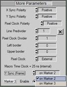
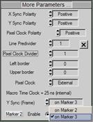
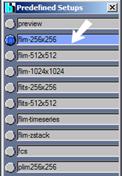
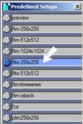
Fig. 3: Left and second left: Clock source selection for FLIM and FLITS. Second right and right: Selection of FLIM mode and FLITS mode from the Predefined Setup pane.

The additional input for the FLITS trigger is provided by a FLITS adapter that is connected between the scan clock cable and the 15 pin sub-D connector of the SPC module, see Fig. 4.

Fig. 4: Clock connection diagram. The FLITS adapter provides an input of the FLITS trigger to Marker 3

Chlorophyll transients

To demonstrate fluorescence lifetime-transient scanning we used the chlorophyll transients that occur when a live plant is exposed to a sudden increase in light intensity [6]. Upon illumination, the fluorescence lifetime (and intensity) first increases. The increase happens within a few milliseconds or tens of milliseconds. It is attributed to the progressive saturation of photosynthesis channels, and a corresponding decrease in fluorescence quenching. The corresponding increase in the fluorescence quantum efficiency (and in the fluorescence lifetime) is called photochemical transient.

After a few seconds of exposure, the fluorescence lifetime starts to decrease again. At intensities comparable to sunlight, it reaches a steady-state level after a few tens of seconds. It is assumed that this slow decrease in the fluorescence lifetime is a protection mechanism of the plant. The slow decrease is called non-photochemical transient.

Non-Photochemical Transient

Recording the non-photochemical transient is relatively easy: It can even be recorded by normal time-series FLIM [2, 3, 4]. To record the transients by FLITS we used a bh DCS‑120 confocal scanning FLIM system [3]. The sample was a fresh grass blade. An appropriate position of the line scan in the sample area was selected in the Preview mode of the DCS system. The excitation intensity during the preview was kept low so that no noticeable lifetime change was induced.

Then the setup was changed to FLITS. This changes the frame clock source to the FLITS trigger, and switches the scanner in the Line mode. The recording was started by generating a single frame clock pulse. The excitation laser was switched on 180 ms later. The result for a line time of 60 ms is shown in Fig. 5.

The horizontal coordinate is the distance along the scanned line, the vertical coordinate is the time, T, after the frame clock. The line time was 60 ms, the number of lines along the T axis is 256. Thus, the total time along the vertical axis is 15.4 seconds. It can clearly be seen that both the fluorescence intensity and the fluorescence lifetime decrease with the time of illumination.

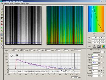
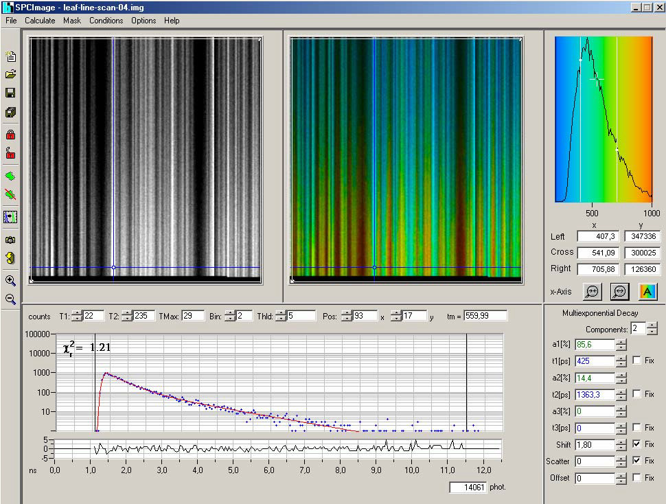
Fig. 5: FLITS image of non-photochemical chlorophyll transient. Horizontal: Distance along the line scanned. Vertical, bottom to top: Time, T, after the start of illumination. 256 pixels along the line, line time 60 ms, 256 lines, total time interval recorded 15.36 seconds. Left: Intensity image. Right Lifetime image. Colour represents lifetime, blue to red corresponds to 200 ps to 1 ns. Amplitude-weighted lifetime of double-exponential decay model. Bottom: Decay curve at cursor position.

The effect is shown in detail in Fig. 5. It shows decay curves for three selected pixel of the line scan for times of 0.5 s, 7.5 s, and 13.4 s after the turn-on of the laser. The mean lifetimes, tm, obtained from a double-exponential fit are 560 ps, 385 ps, and 311 ps, respectively. The changes in the decay profiles are clearly visible.

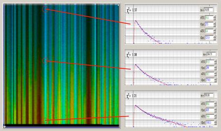
Fig. 6: Decay curves for a selected pixel within the line for times of 0.5 s, 7.5 s, and 13.4 s after the turn-on of the laser

For comparison, a normal lifetime image of the sample is shown in Fig. 7. It was recorded immediately after the FLITS experiment. It can be seen that the sample had not fully recovered from the non-photochemical transient yet: The fluorescence lifetime in the vicinity of the scanned line (horizontal cursor) is still shorter than in the areas nearby.

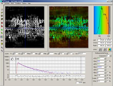
Fig. 7: Fluorescence lifetime image of grass blade, taken after FLITS experiment. Horizontal cursor shows position of the FLIS scan. Intensity image shown left, lifetime image shown right. Coulour represents lifetime, scale from 200 ps to 1 ns. Decay curve at cursor position shown at the bottom.

Photochemical Transient

Recording the photochemical transient requires periodical stimulation and acquisition of the data over a larger number of stimulation periods. Both the laser on-off signal [5] and the frame clock were therefore generated by a bh DDG-210 pulse generator card [2]. The on-off period was 1 second, the on time within the period 200 ms. Each turn-on of the laser initiates a photochemical transient, i.e. a transient increase in the fluorescence lifetime. In the laser-off period the leaf partially recovers, so that the next laser-on initiates a new transient. The total acquisition time was 40 seconds, i.e. 40 on-off periods were accumulated.

The result is shown in Fig. 8. The intensity image is shown on the left, the lifetime image on the right, and a decay curve at the cursor position at the bottom. The horizontal axis of the images is the distance along the line scanned. The vertical axis (bottom to top) is the time after the start of axis. The line time was 1 ms. 256 lines, i.e. 256 ms in total, were recorded along the T direction. The Laser was turned on at T=0, and turned off at T=200 ms. The lifetime image shows the amplitude-weighted lifetime obtained by a double-exponential fit. The lifetime range is from 450 ps (blue) to 650 ps (red).

Although the lifetime change is less pronounced than for the non-photochemical transient an increase can clearly be seen. Changes occur especially in the first 10 to 20 ms after the turn-on of the laser, see bottom of the FLITS image.

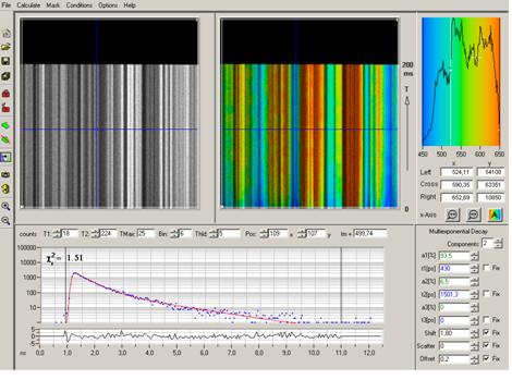
Fig. 8: FLITS image of photochemical chlorophyll transient. Horizontal: Distance along the line scanned. Vertical, bottom to top: Time, T, after the start of illumination. Line time 1 ms, 256 lines, total time interval recorded 256 ms. Laser turned on at T=0, laser-on time 200 ms. Left: Intensity image. Right Lifetime image. Colour represents lifetime, blue to red corresponds to 450 ps to 650 ps. Amplitude-weighted lifetime of double-exponential fit. Bottom: Decay curve at cursor position.

Decay curves and lifetimes for a selected pixel in the scan and for two points on the T axis are shown in Fig. 9. From T = 3 ms to T = 191 ms the amplitude-weighted lifetime of the double-exponential fit increases from 480 ps to 530 ps.

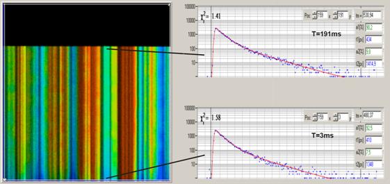
Fig. 9: Decay curves for a selected pixel (x=159) within the line for T=3ms and T=191ms into the laser-on phases. Double-exponential fit. The amplitude-weighted lifetime increases from 480 ps to 530 ps

Despite of the small duty cycle of the laser the illumination necessarily also causes a non-photochemical transient. When the photochemical transient is complete, activity essentially shuts down, and no non-photochemical transient is observed any more. Perfect recording of the photochemical transient therefore requires optimisation of the laser intensity, the laser duty cycle, and the total accumulation time.

Summary

FLITS records fluorescence-lifetime transients at a time scale down to about one millisecond with spatially one-dimensional resolution. Technically, FLITS is obtained by line scanning and replacing the frame clock of a TCSPC FLIM system with a trigger pulse from the stimulation of the lifetime change in the sample. The technique can thus easily be implemented in confocal or multiphoton laser scanning microscopes [3, 4], provided these are able to run a fast line scan. The technique works both for single-shot stimulation, or for periodic stimulation. For a given photon detection rate, the lifetime accuracy for single-shot stimulation decreases with decreasing time-channel width along the transient-time axis. This is not the case for periodic stimulation: Here the accuracy depends on the total acquisition time. Periodic stimulation is thus the key to high fluorescence-transient resolution. Potential applications of FLITS are experiments of plant physiology, electro-physiology, and Ca⁺⁺ imaging of neuronal tissue.