FLIM at a Time-Channel Width of 300 Femtoseconds

For many years, TCSPC FLIM has been performed with 256 time channels and a time-channel width on the order of 50 ps. With the introduction of faster detectors the number of time channels was increased to 1024 and the channel width decreased to 10 ps. Recently, bh have introduced detectors with sub-20 ps IRF width. The Nyquist criterion suggests that FLIM data with these detectors should be recorded with a channel width of about 2 ps. To extract ultra-fast decay components hidden in the detector response even smaller time-channel width can be useful. Here, we report on extracting ultra-fast decay components from FLIM data recorded with a time-channel width of 300 femtoseconds. We show that the components of triple-exponential decay decay functions are reliably resolved down to component lifettime of less than 10ps.

Keywords: FLIM, TCSPC, IRF, Ultra-Fast Fluorescence Decay

Related Applications

TCSPC FLIM

Related Application Notes

Download PDF

FLIM at a Time-Channel Width of 300 Femtoseconds

Wolfgang Becker, V. Shcheslavskiy, Axel Bergmann

Becker & Hickl GmbH

Abstract: For many years, TCSPC FLIM has been performed with 256 time channels and a time-channel width on the order of 50 ps. With the introduction of faster detectors the number of time channels was increased to 1024 and the channel width decreased to 10 ps. Recently, bh have introduced detectors with sub-20 ps IRF width. The Nyquist criterion suggests that FLIM data with these detectors should be recorded with a channel width of about 2 ps. To extract ultra-fast decay components hidden in the detector response even smaller time-channel width can be useful. Here, we report on extracting ultra-fast decay components from FLIM data recorded with a time-channel width of 300 femtoseconds.

Time-Channel width of TCSPC FLIM

For many years TCSPC FLIM data were recorded at a resolution of 256 time channels on the time axis [1]. At a typical observation-time interval of 12 ns 256 time channels gave a time-channel width of about 50 ps. Detectors used at this time, such as the Hamamatsu H7422-40 or the Hamamatsu H5773 and H5783 delivered IRF widths of about 300 ps and 180 ps full width at half maximum (fwhm), respectively [1]. With 50-ps channels, the instrument response functions (IRFs) of these detectors were considered to be sufficiently sampled to fulfil the Nyquist criterion. Under Nyquist conditions, the result of FLIM data analysis does not depend on the relative location of the data points on the IRF or on the rising edge of the fluorescence pulse. Higher numbers of time channels were therefore considered 'empty' resolution, wasting only data space and data-analysis time.

The requirements changed with the introduction of the bh HPM-100-40 hybrid detectors [1, 2, 3]. FLIM systems with these detectors deliver a system IRF of 100 to 140 ps, fwhm, depending on the excitation pulse width. bh therefore moved to a standard FLIM format of 1024 time channels. The time-channel width for a 10-ns recording interval is then about 10 ps. That means the IRF is sampled with 10 or more data points, and the Nyquist criterion is, again, satisfied. Of course, the four-fold increase in the number of time channels leads to a similar increase in data size, and, consequently, in FLIM data processing time. bh therefore implemented GPU processing in the data analysis software. GPU processing speeds up the data analysis by a factor of 100 so that data processing time is no longer a problem [4].

Recently, bh have introduced FLIM systems with SPC-150NX and HPM-100-06 detectors [1, 5]. With femtosecond excitation, these systems deliver IRF widths smaller than 20 ps, fwhm [6]. That means a time-channel width of 2 ps or less should be used to satisfy the Nyquist criterion, and the number of time channels should be increased to 4096. It could be objected that distributing the photons over a number of channels this large would result in a smaller number of photons per channel and, consequently, in a decrease of the accuracy of the FLIM data analysis. This is, however, not the case. The signal-to-noise ratio of the lifetime is independent of the number of time channels, as has been shown in [7]. It only depends on the total number of photons. Three examples of FLIM decay traces recorded with different FLIM data formats are shown in Fig. 1.

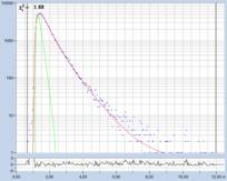
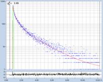
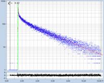
Fig. 1: Decay curves from FLIM data with different time-channel width. Left to right: 50 ps, 12 ps, and 2.4 ps. Recording-time interval 12.5 ns. The red curve is a fit with a three-component model. (Data from different samples)

A time-channel width on the order of 2 ps does not pose a problem to the bh TCSPC / FLIM modules - it can even be reached with early modules, such as the SPC-830. However, just covering the IRF width with enough data points is not all. High-resolution FLIM systems may be used to extract ultra-fast decay components with lifetimes shorter than the IRF width. Such decay components are more frequent than commonly believed. We have found them in mushroom spores, plant tissue, mammalian hair, and in malignant melanoma [8, 9, 10]. The components can have decay times down to 7 ps, perhaps even less. In these cases not only the IRF but also the decay function must be adequately sampled. Consequently, time-channel widths below 700 fs should be used in these cases. Channel widths in this range are available from the SPC-180NX, the SPC-180NXX, and the equivalent SPC-150NX and -NXX versions [1].

Effect of the Channel Width on the Resolution of the Decay Components

To demonstrate the effect of different time-channel width on the resolution of fast decay components we recorded lifetime images of mushroom spores with our DCS-120 MP fibre-laser multiphoton system [6]. The detector was a HPM-100-06 module, the TCSPC module an SPC-180NXX. Two-photon images at 780 nm excitation wavelength were taken from spores of Paxillus involutus, IRFs were recorded by taking SHG images of finely powdered sugar. All data were recorded through a non-descanned detection path. Scattered laser light was blocked by Chroma SP680 filters. The emission filter for the FLIM recordings was a 450-nm long pass. For IRF recording the filter was taken out. Pairs of fluorescence images and SHG images were recorded with a time-channel width of 3 ps and 300 fs. The total number of time channels was 4096 in both cases, covering observation-time intervals of 12.5 ns and 1.25 ns, respectively. Raw data from SPCM data acquisition software are shown in Fig. 2. An ultra-fast decay component is clearly visible in the data.

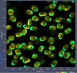
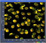
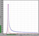
Fig. 2: Paxillus involutus spores, raw data in SPCM. Images, decay curves (blue) and IRFs (red), 3 ps / channel and 300 fs / channel. Displayed by online display functions of SPCM data acquisition software, linear scale.

Precision FLIM analysis was performed by bh SPCImage NG FLIM data analysis software [1, 4]. In all cases, triple-exponential decay analysis was applied to the data. Data recorded with 3 ps channel width are shown in Fig. 3. An image of the fastest decay component, t1, is shown on the left, a decay curve at the cursor position in the middle. The insert in the decay window shows the amplitudes and the lifetimes of the decay components. A histogram of the t1 values over all pixels of the image is shown on the right.

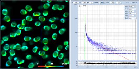
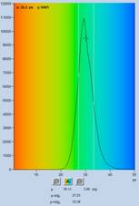
Fig. 3: Spores of Paxillus involutus, time-channel width 3 ps, 4096 time channels, observation-time interval 12.5 ns. Left to right: Image of fastest decay component, t1, decay curve at cursor position (blue) and IRF (green), histogram of t1 values over the pixels of the image. Auto IRF of SPCImage NG.

As can be seen from the figure, a good fit of the decay data is obtained. The lifetime of the fast component, t1, is obtained at high signal-to-noise ratio, as the t1 image and the histogram show. The most frequent value of t1 is about 30 ps.

For the analysis shown above the 'auto' IRF of SPCimage was used, please see [1], chapter 'SPCImage NG Data Analysis Software'. Experience has shown that for extremely fast decays the 'auto' IRF often comes out a bit too short. Therefore we analysed the same data with a real (measured) IRF. The result is shown in Fig. 4. The figure shows that the general composition of the decays remains the same, with the difference that t1 becomes a bit shorter. However, considering the fact that the lifetime is on the on the order of only 25 ps, the difference is not significant. Nevertheless, analysis of further data with femtosecond time-channel width was performed with the real IRF.

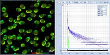
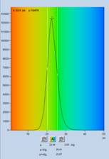
Fig. 4: Same as in Fig. 3, but analysed with the real IRF.

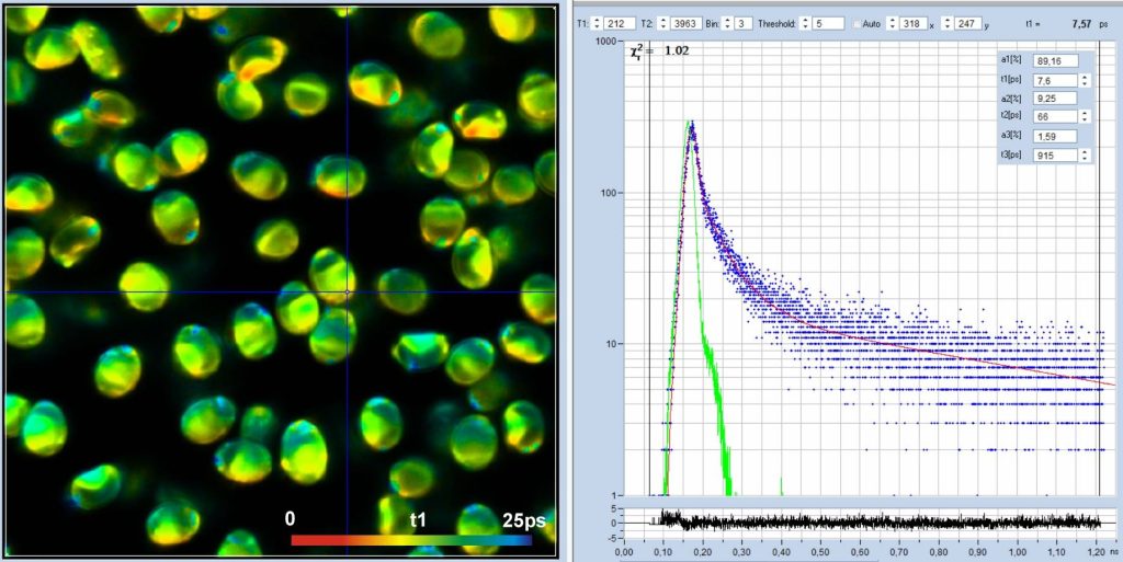
Fig. 5 shows data recorded with a time-channel width of 300 femtoseconds, i.e. on a time scale 10 times faster than in Fig. 3 and Fig. 4. The number of time channels is 4096, the total observation-time interval 1,25 ns. The decay data in a selected spot are shown in the middle. The green curve is the IRF, the blue dots are the photon numbers in the time channels. The IRF is a real one, recorded from powdered sugar. At the time scale used, the fwhm of the IRF extends over 70 data points. The figure resembles a decay/IRF plot from a conventional lifetime spectrometer, with the difference that the time scale is 20 times faster. With the data resolved into a number of data points this high, the deconvolution routine is able to determine lifetime components considerably shorter than the IRF width. In the data shown in Fig. 5 the fast component, t1, of the 3-ps data is split into two, with a t1 around 13 ps and a low-amplitude component, t2, of about 60 ps. The distribution of t1 is shown in the histogram on the right of Fig. 5.

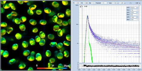
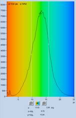
Fig. 5: Spores of Paxillus involutus, time-channel width 300 fs, 4096 time channels, observation-time interval 1.25 ns. Left: Image of the fast decay component, t1, colour scale 0 to 25 ps. Middle: Decay curve (blue), IRF (green), and decay parameters at the cursor position. Right: Histogram of the t1 values over the pixels of the image.

Discussion

The results shown above demonstrate that FLIM systems with the -NXX versions of the bh TCSPC/FLIM modules and HPM-100-06 detectors are able to resolve decay components in the sub‑10ps range. This does not mean, however, that measurements in the ultra-fast decay domain are straightforward. A frequent problem are reflections in the NDD beam path of the microscope. To collect photons which are scattered on the way out of the sample a lens projects an image of the microscope lens on the detector. Usually even a two-step projection is used: A first lens projects an image of the microscope lens on a second lens in front of the detector. The second lens projects an image of the first lens on the active area of the detector. This design has the advantage that the diameter of the beams can be kept smaller, and that a roughly parallel part of the beam is available in which filters can be placed. However, the principle is prone to optical reflections. Photons reflected at the detector or another optical surface are likely to be projected back onto another surface, reflected a second time, and fed back to the detector some 10 or 100 ps later. The result are ugly reflections in the decay curves. In data with ultra-fast components of high amplitude the problem is enhanced by the high intensity ratio between the peak and the later part of the decay curves. In the NDD light path of the DCS-120MP system the problem has been accounted for by carefully selecting lens curvatures to avoid collimated reflection from the lens surfaces.

Moreover, the design of the non-descanned optics does not automatically guarantee that the optical path length is constant for beams of all angles and over the entire aperture. The most critical element is the lens in front of the detector. This lens has a short focal length and a large diameter. Thus it has a large amount of spherical aberration. That means rays entering the lens at the periphery and the centre have different effective path length and different transit times. The differences can be on the order of a few picoseconds. In our system the effect causes a slight increase of the IRF width, from 18 to 19 ps fwhm in a free beam to about 23 ps in the NDD beam path. In first approximation, the broadening is the same for the fluorescence measurement and the IRF measurement. It has thus little influence on the results. Changes can, however, occur if the sample is not correctly focused or if microscope lenses are changed. In these cases the intensity distribution over the beam cross section and, consequently, the transit time distribution change.

Another potential problem is related to IRF measurement. There is no other way than to measure the IRF via an SHG process. At first glance this appears to be an ideal solution. SHG is (within the resolution of the system) infinitely fast, and it is emitted at high intensity. Possible contamination with fluorescence therefore has little effect on the result. Nevertheless, there is a problem. SHG is emitted in forward direction. Normally, enough light from within the sample is scattered back into the detection beam path. However, light leaving the sample at the back can be reflected or scattered back, and transferred to the detector. The reflected light arrives with a delay and thus broadens the recorded IRF or causes nasty secondary pulses. It is therefore important to cover the back of the sample with an absorbent cover. But even then, an unknown portion of the signal can come back from the cover. Taking into account that the forward emission is much stronger than the backward emission an influence on the recorded IRF shape cannot entirely be excluded. All in all, attention to the optical details is recommended when ultra-high resolution FLIM data are recorded.