TCSPC System Records FLIM of a Rotating Object

Wolfgang Becker, Holger Netz, Becker & Hickl GmbH, Berlin, Germany

Abstract: We describe a setup for fluorescence lifetime imaging of a three-dimensional object. The object is rotated around a vertical axis and simultaneously scanned vertically by a fast galvanometer scanner. The excitation light comes from a BDS-SM picosecond diode laser. FLIM is recorded by a standard SPC-150 TCSPC module via the normal multidimensional recording process of the bh TCSPC devices. The resulting image is a developed view of the entire sample surface, containing a full fluorescence decay curve in each pixel.

Motivation

Small-animal tomography techniques - no matter whether optical or non-optical - often use rotation of the measurement object to obtain data for different projection angles. Although such techniques are not normally focusing on fluorescence lifetime detection they can be favourably supplemented by recording time-resolved data, especially fluorescence lifetime images or time-resolved diffuse reflection images. The fluorescence lifetime delivers direct information on molecular parameters, and time-resolved diffuse reflection data deliver scattering and absorption parameters from different tissue layers [1, 2, 3]. In this application note we show how fluorescence lifetime images of the entire circumferential surface of a rotating object can be obtained by bh's multi-dimensional TCSPC technique.

Principle

The optical principle is shown in Fig. 1. The object is placed on a table which rotates it around its vertical axis. Simultaneously, the object is scanned vertically by a fast galvanometer mirror. A bh BDS-SM picosecond diode laser is used for exciting fluorescence in the object [4]. The pulse repetition rate of the laser is 20, 50, or 80 MHz. Due to the high repetition rate the pulsing of the laser does not interfere with the scanning. A lens, L1, focuses the laser beam into an intermediate image plane. A projection lens system, L2 and L3, projects this plane on the surface of the object. As the galvanometer mirror is moving, the laser spot moves up and down the surface of the object. With the rotation of the table, the entire surface of the object is scanned by the laser spot. Fluorescence emitted at the object is projected back into the intermediate image plane and collimated by L1. It is separated from the excitation light by a dichroic mirror. It then passes a long-pass or bandpass filter that removes residual laser light and is detected by a single-photon sensitive detector.

The single-photon pulses from the detector are fed into the 'CFD' input of the TCSPC module. The timing reference (SYNC) signal for the TCSPC module comes from the laser. The imaging process in the TCSPC module is synchronised with the rotation of the table and the vertical scanning by frame clock, line clock, and pixel clock pulses [1]. The frame clock is picked up from the table by a magnetic sensor, the 'line' and 'pixel' clocks come from the controller of the galvanometer mirror.

FLIM recording is performed by the normal multi-dimensional recording process of the bh TCSPC devices [1, 2]. Single photons from the illuminated spot are detected, the times of the photons after the laser pulses are determined, and a photon distribution over these times and the vertical position of the laser beam and the rotation angle in the moment of the photon detection is built up. The result is a developed image of the entire surface of the object, containing a fluorescence decay curve in every pixel.

Fig. 1: Principle of the optical system

System components

For demonstrating the principle described above we used a bh SPC-150 TCSPC/FLIM module, a GVD-120 scan controller card, a DCC-100 detector controller, and a PMC-150-20 cooled PMT module [1]. The SPC-150, the GVD-120 and the DCC-100 were operated in a 'Simple-Tau' extension box connected to a laptop computer [1]. The optical system was assembled from standard Thorlabs parts and standard lenses. The excitation light was delivered by a bh BDS-SM-473nm picosecond diode laser [4]. Vertical scanning was performed by a Thorlabs GPS011 scanner with a CB74EX scan motor. The object was rotated by a Faulhaber Series 1512-012SR 324:1 DC motor. The speed of the motor was about 1 rotation in 5 seconds. The entire system is shown in Fig. 2.

Fig. 2: Imaging setup, with laser, TCSPC system, and optical system

Operating Software

The entire system was controlled by version 9.78 bh SPCM TCSPC data acquisition software [1, 5]. SPCM includes measurement control, scanner and laser control, detector control, and online display of intensity images, lifetime images, and decay curves. The user interface configured for the experiments described here is shown in Fig. 3.

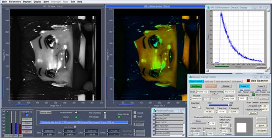
Fig. 3: User interface of the bh SPCM TCSPC data acquisition software

Test Result

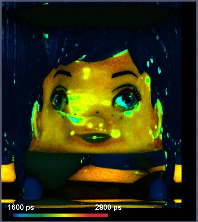
We tested our setup with the test object shown in Fig. 4, left. A lifetime image provided online by SPCM software is shown in Fig. 4, middle. The lifetime range is from 1000 ps (blue) to 3000 ps (red). A decay curve in a selected spot of the image is shown in Fig. 4, right.

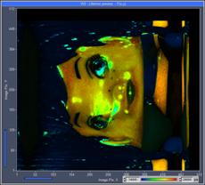
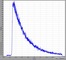
Fig. 4, left to right: Test object, lifetime image, decay curve in selected spot. 512 x 512 pixels, 1024 time channels per pixel. Image and decay curve created by online display functions of SPCM data acquisition software [5, 6].

The data shown in Fig. 4 were recorded with a laser power of about 100 µW. The average count rate at this laser power was about 400,000 s^-1 on average, and about 900,000 s^-1 in the bright areas. The acquisition time was about one minute, i.e. photons from 12 rotations of the object were accumulated.

Data Analysis with SPCImage

Double and triple-exponential decay analysis in the time domain and phasor data analysis in the frequency domain can be performed as usual with SPCImage FLIM analysis software [1, 7]. Data are sent from SPCM to SPCImage by the 'Send data to SPCImage' command. The main panel of SPCImage with the data from Fig. 4 is shown in Fig. 5, left, a phasor plot of the same data in Fig. 5, right.

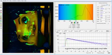
Fig. 5: Left: Main panel of SPCImage data analysis software with FLIM data of test object loaded. Right: Phasor plot of the same data.

Concluding Remarks

The setup described in this note provides a relatively simple and inexpensive way to record lifetime images of the entire circumferential surface of a three-dimensional object. A few non-ideal features should, however, be taken into regard.

The first one is that the path length to the surface of the object and back varies with the surface topography. One millimeter variation in surface topography causes 2 mm path length difference, and thus a difference of 6.6 ps in transit time. The transit time difference transfers directly into a shift in the measured fluorescence lifetime. The problem can, in principle, be solved by using a floating IRF in SPCImage. However, a floating IRF increases the noise in the calculated lifetime, especially for fast decay components in the range of the IRF width.

Another feature is the low collection efficiency of the optics. For a given diameter of the galvanometer mirror, there is a reciprocal relationship between the maximum diameter of the scan area and the numerical aperture of the light collection. The light collection efficiency is therefore lower than in a scanning system with a microscope [1]. However, different than in microscopy, the excitation light is distributed over a large scan area. The excitation dose per area unit is therefore much lower. Consequently, photobleaching and photodamage are far less a problem. The low collection efficiency can therefore partially compensated by using higher excitation power.

References

1.            W. Becker, The bh TCSPC handbook. Becker & Hickl GmbH, 7th ed. (2017). Available on www.becker-hickl.com. Please contact bh for printed copies.

2.            W. Becker, Advanced time-correlated single photon counting techniques. Springer, Berlin, Heidelberg, New York (2005)

3.            H. Wabnitz, J. Rodriguez, I. Yaroslavsky, A. Yaroslavsky, and V. V. Tuchin, Time-Resolved Imaging in Diffusive Media, in: Handbook of Optical Biomedical Diagnostics, Second Edition, Volume 1: Light-Tissue Interaction (SPIE PRESS, 2016), pp. 397–475.

4.            Becker & Hickl GmbH, BDS-SM family picosecond diode lasers. Extended data sheet, available on www.becker-hickl.com

5.            Becker & Hickl GmbH, New SPCM Version 9.78 comes with new software functions. Application note, available on www.becker-hickl.com

6.            Becker & Hickl GmbH, SPCM Software runs online-FLIM at 10 images per second. Application note, available on www.becker-hickl.com

7.            Becker & Hickl GmbH, New SPCImage Version Combines Time-Domain Analysis with Phasor Plot. Application note, available on www.becker-hickl.com