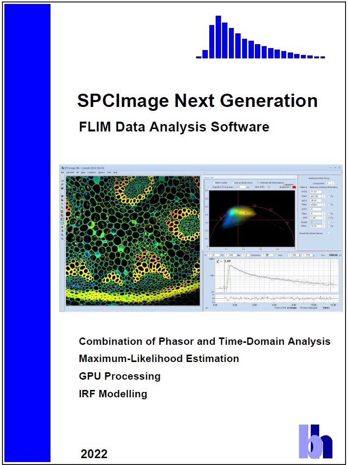
SPCImage NG FLIM Data Analysis Software
Abstract: SPCImage
NG is a new generation of bh's TCSPC-FLIM data analysis software. It combines
time-domain and frequency-domain analysis, uses a maximum-likelihood algorithm
to calculate the parameters of the decay functions in the individual pixels,
and accelerates the analysis procedure by GPU processing. 1D and 2D parameter
histograms are available to display the distribution of the decay parameters
over the pixels of the image or over selectable ROIs. Image segmentation can be
performed via the phasor plot and pixels with similar signature be combined for
high-accuracy time-domain analysis. SPCImage NG provides decay models with one,
two, or three exponential components, incomplete-decay models, and
shifted-component models. Another important feature is advanced IRF modelling,
making it unnecessary to record IRFs for the individual FLIM data sets.
Principle
SPCImage NG produces colour-coded images of
fluorescence lifetimes and other fluorescence decay parameters from TCSPC FLIM data. It runs an iterative fit and de-convolution procedure on the decay data of
the individual pixels of the FLIM images. In the simplest case, the result is
the lifetime of the decay functions in the individual pixels. For complex decay
functions the fit procedure delivers the lifetimes and amplitudes of the decay
components. SPCImage then creates colour-coded images of the amplitude- or
intensity-weighted lifetimes in the pixels, images of the lifetimes or
amplitudes of the decay components, images of lifetime or amplitude ratios, and
images of other combinations of decay parameters, such as FRET intensities,
FRET distances, bound-unbound ratios, metabolic indicators, or the
fluorescence-lifetime redox ratio, FLIRR. Examples are shown in Fig. 1 through Fig.
6.
Fig. 1: Image
of the amplitude-weighted lifetime, tm, of a double-exponential decay. Right:
Fluorescence decay curves in selected pixels.
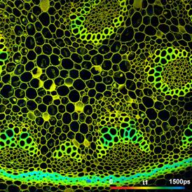
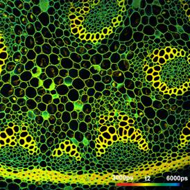
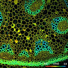
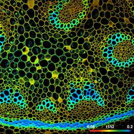
Fig. 2: Upper row: Images of the lifetimes of the fast component, t1, and
the slow component, t2, of a double-exponential decay. Lower Row: Images of the
amplitude ratio, a1/a2, and the lifetime ratio, t1/t2, of the fast and the slow
decay component.
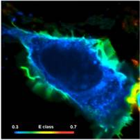

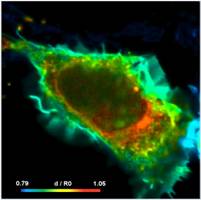
Fig. 3: FRET imaging. Cell with
interacting proteins, labelled with a FRET donor and a FRET acceptor. Left to
right: Classic FRET efficiency, FRET efficiency of interacting donor fraction,
FRET distance
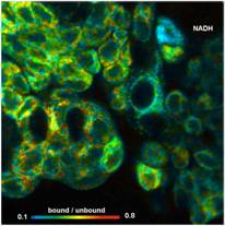
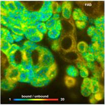
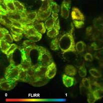
Fig. 4: Metabolic FLIM on the cell level. Bound-unbound ratio of NADH,
Bound/unbound ratio of FAD, Fluorescence-Lifetime Redox Ratio, FLIRR.
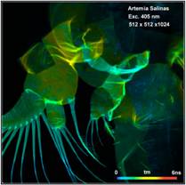
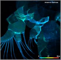
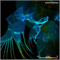
Fig. 5: Autofluorescence FLIM of small
organisms. Artemia salinas, amplitude-weighted lifetime, tm, lifetime of
fast decay component, t1, amplitude ratio of fast and slow component (metabolic
ratio), a1/a2.
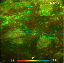
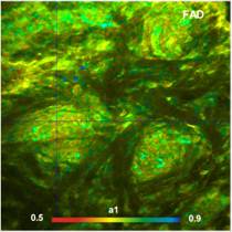
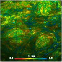
Fig. 6: Two-photon deep-tissue metabolic FLIM. Mammalian skin, NADH and
FAD images, metabolic indicator a1 and FLRR image.
GPU Processing
bh FLIM data can contain an enormous number
of pixels and time channels. Images with 1024 x 1024 or even 2048 x
2048 pixels are not uncommon, and time-channel numbers of 1024 are routinely
used in combination with the bh HPM-100-40 detectors [2]. Such data sets are
equivalent to a stack of 1024 One-Megapixel images. Processing such amounts of data
by the CPU of even a fast computer can take tens of minutes. SPCImage NG therefore
uses GPU (Graphics Processor Unit) processing. The TCSPC data are transferred
into the GPU, which then runs the de-convolution and fit procedure for a large
number of pixels in parallel. This way, data processing times are reduced from
formerly several minutes to a few seconds. The short processing time not only
simplifies the processing of larger series of data set from a given experiment,
it also makes it easy to select the best data sets from a given experiment, or run
the analysis with different decay models or different IRF models to find the
best way to process them. GPU processing is running on all NVIDIA cards and a
number of other NVIDIA-compatible display devices. When SPCImage NG finds a
suitable device in the computer it automatically runs the data analysis on it.
Fig. 7: Left: Progress panel during
lifetime calculation, showing that GPU processing is used. Right: Part of
'Preferences' panel, indicating that a Quadro K1100M CUDA 7.0 device was found.
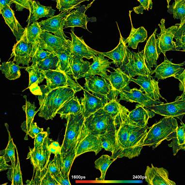
Fig. 8: A lifetime image with 1024 x 1024
pixels and 1024 time channel per pixel. The image was calculated on an NVIDIA
GPU in 10 seconds. Recorded by bh FASTAC FLIM system on a Zeiss LSM 880
NLO.
Phasor Plot
SPCImage FLIM analysis software combines
time-domain multi-exponential decay analysis with phasor analysis [15]. Phasor
analysis expresses the decay data in the individual pixels as phase and
amplitude values in a polar diagram, the 'Phasor Plot'. Pixels with similar
decay signature form distinct clusters in the phasor plot. Clusters of interest
can be selected and back-annotated in the lifetime image for further processing
or for combination of pixel data. An example is shown in Fig. 9.
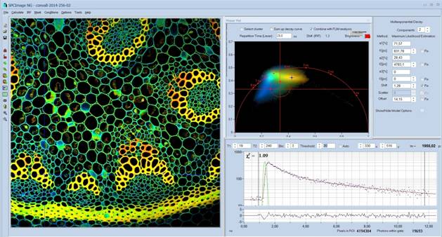
Fig. 9:
Combination of time-domain analysis (left and lower right) and Phasor Plot (upper right)
Image Segmentation by Phasor Plot
Selection of pixels with an interesting
phasor signature is demonstrated in Fig. 10. It shows a lifetime image of a
tumor in a mouse, the corresponding phasor plot with selection of the phasor
range of the tumor, and back-annotation of the pixels within the selected phasor
range in the image.
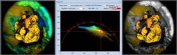
Fig. 10: Left to right: Lifetime image of a mouse tumor, phasor plot with
selection of the phasor range of the tumor, and back-annotation of the pixels
with the selected phasor signature in the image.
The procedure described above can be used
in images containing a large number of cells in the same field of view, as
shown in Fig. 11. Cell compartments with different decay signature form
separate clusters in the phasor plot. Interesting clusters are selected by the 'Select
Cluster' function and back-annotated in the images as shown in Fig. 12 and Fig.
13. A single decay curve can be built up for the combined pixels inside the
phasor cluster selected. This curve contains a high number of photons and can
be used for precision multi-exponential decay analysis.
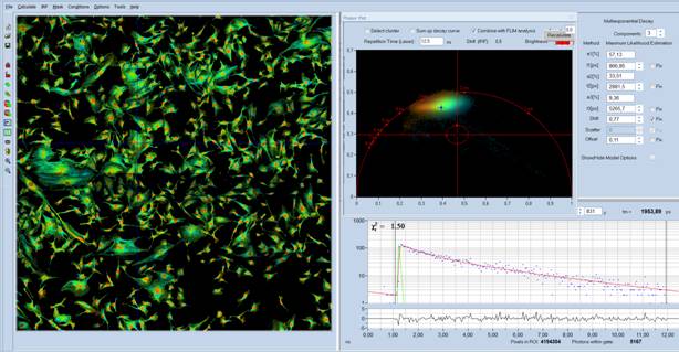
Fig. 11: Spatial Mosaic FLIM image showing a large number of cells. The
phasor plot (upper right) displays distinct clusters for the nuclei and the
cytoplasm.
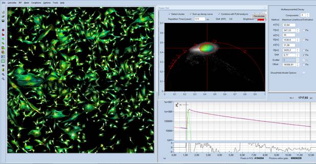
Fig. 12: The cytoplasm of the cells has been selected by the 'Select
Cluster' Function. A combined decay curve for the selected pixels is displayed
by the 'Sum up decay curves' function.
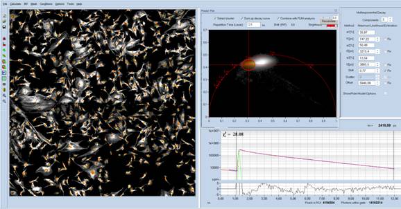
Fig. 13: The nuclei of the cells have been selected by the 'Select Cluster'
Function. The histogram (shown right) refers to the selected pixels. A combined
decay curve for the selected pixels is displayed by the 'Sum up decay curves'
function.
Precision Decay Analysis of Moving Objects
Precision lifetime imaging of live objects
is often hampered by motion in the sample. To avoid that details are smeared
out it is often attempted to record the FLIM data in a single, fast scan. This
approach is not very successful. It usually results in low photon numbers in
the pixels, making precision multi-exponential analysis impossible. The bh
TCSPC systems solve the problem by recording a 'temporal mosaic'. That means a
series of fast scans is performed and the data are written in subsequent elements
of a data mosaic [1, 8]. The
entire mosaic is then loaded into SPCImage NG, and a preliminary data analysis
is performed. The data are loaded into the phasor plot, the phasor signature of
the detail of interest is selected, and the selection is back-annotated in the
mosaic image. Combination of the pixels yields a single decay curve with a
large number of photons. Fig. 14 demonstrates the procedure at the example of a
live water flee. The decay curve of the combined pixels is shown lower right,
the decay parameters upper right. Decay analysis shows decay parameters typical
of FAD, with a small contribution of FMN. That means the procedure is able to
perform metabolic FLIM at a moving leg of a water flee!
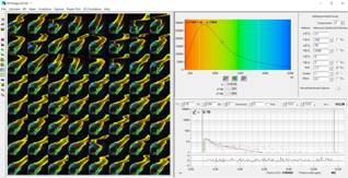
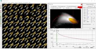
Fig. 14: Temporal-Mosaic FLIM data showing the leg of a live water flee.
Left: The photon number in a single pixel is too low for precision decay
analysis. Right: Selection of the phasor range of interest and combination of
the pixels yields a high accuracy decay curve.
Trajectory of Dynamic Systems in the Phasor Space
Another feature of the phasor plot is that
it displays dynamic changes in the fluorescence-decay behaviour of a sample. An
example is shown in Fig. 15. It shows a temporal-mosaic recording of
chloroplasts in a leaf [1]. The image mosaic (shown left) shows how the
chloroplasts change their fluorescence decay time with the time of exposure.
The phasor plot (shown right) displays the trajectory the system is taking in
the phasor plot. In the present case, the phasor trajectory shows that the
fluorescence decay functions of the chlorophyll for a given time after the
start of the exposure are close to single exponential. This contradicts common
opinion. Obviously, strongly multi-exponential decay reported for chlorophyll
in live plants comes from the dynamic change of the lifetime during the
acquisition time period rather than from intrinsic multi-exponential behaviour.
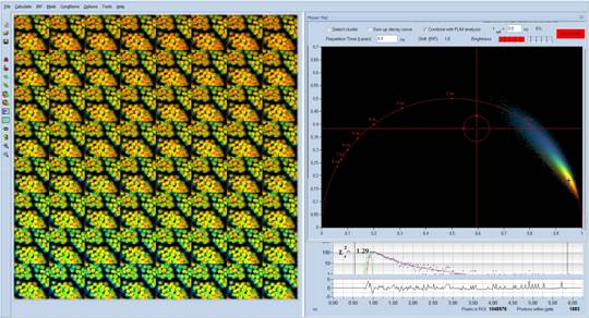
Fig. 15: Temporal-mosaic FLIM of a plant leaf. The Phasor Plot shows the
trajectory the system is taking in the phasor space.
Analysis of Special Data Types
Ultra-Fast FLIM
For many years, TCSPC FLIM has been
performed with 256 time channels and a time-channel width of about 50 ps.
With the introduction of the HPM-100-40 hybrid detectors [2] bh moved to a standard
FLIM format of 1024 time-channels, and a channel with of 10 ps. Recently,
bh have introduced FLIM systems with HPM-40-06 detectors [1, 3]. The systems
have an IRF width of <20 ps, fwhm [5, 6, 7]. To fully exploit an IRF
this fast, the data must be recorded with 4096 time channels and a time-channel
width of 1 ps or shorter. For the determination of component lifetimes in
the range of 20 ps and below even shorter time-channel width is appropriate.
Recent versions of SPCImage NG therefore account for analysis of decay data
with femtosecond time-channel width and 4096 time channels [1, 4]. An example is shown in Fig. 16. The
time-channel width is 300 femtoseconds. With a channel width this small
the IRF (green curve) is sampled with about 70 data points. Together with a
large number of photons and triple-exponential analysis, this allows decay components
down to less than 10 ps to be determined, see histogram of t1, Fig. 16, right.
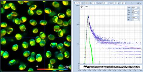
Fig. 16: Ultra-high resolution FLIM of Paxillus
involutus spores [5]. Left
to right: Lifetime image of fastest decay component, t1, decay curve at cursor
position, histogram of t1 over the pixels of the image. Time-channel width 300
femtoseconds, 4096 time channels, IRF width 23 ps, observation-time
interval 1.25 ns. Analysed with real IRF, recorded from powdered sugar.
Triple-exponential decay analysis shows that the fast decay components is in
the range of 13 picoseconds.
Dual-Channel Metabolic FLIM
Metabolic FLIM is increasingly using
wavelength multiplexing in combination with dual-channel detection [1, 9, 10]. This way, NADH and FAD images are
obtained with virtually no spectral crosstalk. Since it is desirable to
cross-calculate ratios of decay parameters between the two channels SPCImage NG
has been extended to hold two FLIM data channels in the memory, and to display
two images simultaneously. For colour coding of the images, ratios of decay
parameters from different channels can be selected. An example is shown in Fig.
17.
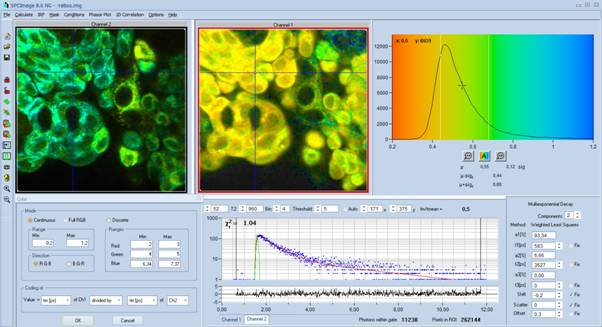
Fig. 17: Dual-channel metabolic FLIM, recorded by wavelength-multiplexed
excitation and recording in separate wavelength channels. NADH image shown
left, FAD image shown right. Both images colour-coded with the ratio of the amplitude-weighted
lifetimes of NADH and FAD.
INT FLIM Data
INT FLIM (Intensity-linear FLIM) is a new
recording mode of the bh SPC-180N family modules. For every pixel, the data
contain the usual decay function with the selected number of time channels together
with the total photon number [1,
11]. The photon number is determined by an additional fast counter channel in parallel
with the timing electronics. The technique delivers high-resolution decay data
with a linear intensity scale. SPCImage NG automatically recognises such data
and handles them accordingly. That means the fit procedure is performed on the
decay data as usual, but the image intensity comes from the photon number in
the fast counter channel. An example is shown in Fig. 18.
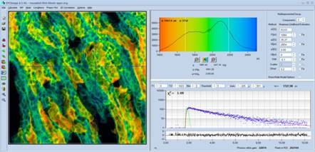
Fig. 18: Data from INT-FLIM recording. INT FLIM data contain decay data
from the TCSPC timing electronics in combination with intensity data from a
fast counter. The technique is used to obtain high-resolution decay data with a
linear intensity scale. SPCImage NG automatically recognises such data and
processes and displays them with the correct time scale and intensity scale.
Simultaneous FLIM / PLIM
The bh FLIM systems are able to record FLIM
and PLIM simultaneously [1, 13]. SPCImage NG loads the entire FLIM/PLIM data
set, and displays both images simultaneously. Please see Fig. 19.
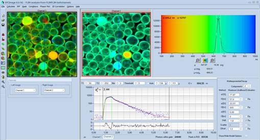
Fig. 19:
Analysis of data from simultaneous FLIM / PLIM experiment. Left FLIM,
right: PLIM. Decay curve and histogram shown for PLIM.
Single-Curve Analysis
Resent versions of SPCImage NG simplify the
analysis of single-curve fluorescence decay data. The data can either be
recorded by scanning a sample solution with a bh FLIM system or by recording a
single curve in a cuvette setup. Analysis is possible with all decay models implemented
in SPCImage, and with a synthetic or a measured IRF. Fig. 20 shows the decay
function recorded from an NADH solution with a fast FLIM system of 20 ps
IRF width.
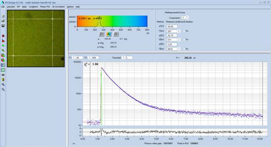
Fig. 20: Fluorescence decay of an NADH solution. Data recorded by FLIM,
pixels within cursor area combined into single decay curve. Triple-exponential
decay analysis with synthetic IRF.
Batch Processing
A batch-processing function is available
for analysing a large number of FLIM data sets automatically. Please see [1], 'The bh TCSPC Handbook', chapter
'SPCImage NG Data Analysis'.
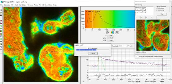
Fig. 21: Batch Processing in progress. Subsequent files are loaded,
analysed, and saved.
Histograms
Decay Parameters
SPCImage has histogram functions for the decay
parameters. The histogram shows how often pixels of a given parameter value
occur in the lifetime image. The parameter histogram is thus an efficient tool
to determine decay parameters in selected regions of interest, get an estimate
of the variance of parameters, and to compare decay parameters of different
samples [5, 12].
The histogram refers either to a selected
region of interest or, if no ROI was defined, to the entire lifetime image.
Together with the various options to select decay parameters and combinations
of decay parameters a wide variety of different histograms can be obtained. A
few examples are shown in Fig. 22 through Fig. 24.
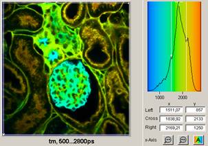
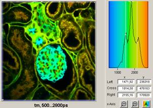
Fig. 22: Histograms of the mean (amplitude weighted) lifetime of
double-exponential fit. Left: Un-weighted frequency of pixels. Right:
Intensity-weighted frequency of pixels. Note that the peak at 1500ps is
enhanced due to high intensities of the pixels, and peak at 2100 ps is reduced
due low intensities.
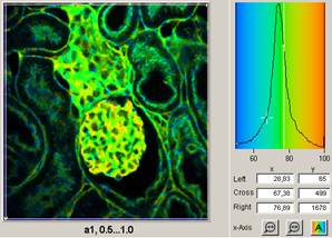
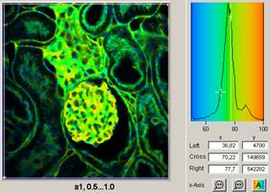
Fig. 23: Histograms of the amplitude, a1,
of the fast decay component. Left: Un-weighted frequency of pixels. Right:
Intensity-weighted frequency of pixels. The peak at 0.85 (85%) is only visible
in the intensity-weighted histogram because it is caused by a small number of
pixels that have high intensity.
SPCImage NG allows the user to define
multiple regions of interest. In that case, every ROI has its own parameter
histogram. The desired ROI and the corresponding histogram can be selected by
the buttons on top of the histograms, or by clicking on the red dot in the
centre of the ROI. An example is shown in Fig. 24.
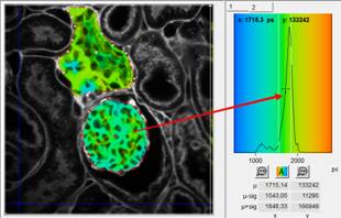
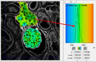
Fig. 24:
Multiple ROIs, selection via the buttons on top of the histograms
2-D Histograms
2D histograms present density plots of the
pixels over two selectable decay parameters. The decay parameters can be
lifetimes, t1, t2, t3, or amplitudes, a1, a2, a3, of decay components,
amplitude or intensity-weighted lifetimes, tm or ti, or arithmetic conjunctions
of these parameters. An example is shown in Fig. 25. A histogram of the amplitude,
a1, of the fast decay component versus the amplitude-weighted
lifetime, tm, has been selected. Cursors in the histogram are available to
select special parameter combinations and highlight the corresponding pixels in
the lifetime image.
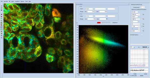
Fig. 25: 2-D histogram showing density plot of pixels over
amplitude-weighted lifetime, tm, and amplitude of fast component, a1.
Intensity Histogram
Instead of the parameter histogram,
SPCImage NG can also display an intensity histogram, see Fig. 26. The cursors
in the intensity histogram interact directly with the 'Intensity' Parameters of
the image display [1]. An example is shown in Fig. 26, right.
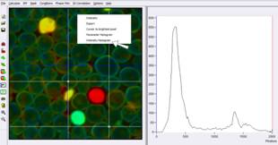
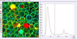
Fig. 26: Intensity Histogram of SPCImage NG. Left: The samplee containeds a
few dead cells with extremely high intensity. Within the entire intensity range
of the image, the cells of interest are displayed only dimply. Right: By pulling
the cursors to the intensity range of the cells of interest results a perfect image
is obtained.
ROIs
SPCImage NG allows the user to define ROIs
in the images. Both rectangular and polygonal ROIs can be defined. Parameter
histograms are displayed for the selected ROI, see Fig. 27.
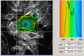
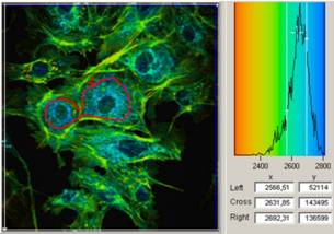
Fig. 27: ROI
Definition. Left: Rectangular ROI. Right: Polygonal ROI
Several polygonal ROIs can be defined, and
the corresponding parameter histograms be selected via the buttons on top of
the histogram window. Please see Fig. 28.
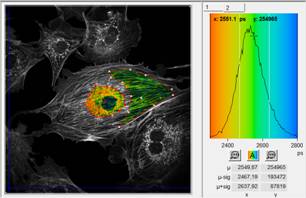
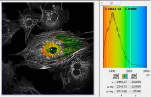
Fig. 28:
Multiple ROIs, with selection of parameter histogram.
Procedures and Algorithms
Intelligent Binning
Microscopy images are over-sampled to
obtain maximum spatial resolution. Oversampling means that the point spread
function is sampled by several pixels in x and y. Typical (linear) oversampling
factors are around 5, that means the point-spread function is sampled by about
25 pixels. Of course, these pixels contain virtually identical lifetime
information. Analysing them individually would result in low photon number per
pixel, and in unnecessarily high noise in the decay parameters. To avoid this
problem SPCImage NG uses overlapping binning of the decay data. The procedure
leaves the number of pixels unchanged but includes decay data from several pixels
around the current one into each calculation step [1, 12]. An example is shown in Fig. 29. The
image on the left shows a scan of 128 x 128 pixels, analysed by
SPCImage NG without binning. The image on the right was recorded with
512 x 512 pixels. Photon rate and acquisition time were the same. To
compensate for the lower number of photons per pixel the data were analysed using
a binning are of 5 x 5 pixels. This brings the photon number to the
same level as in the 128 x 128 image. The effect is striking: The
spatial resolution is massively improved, but there is no blur-out of the lifetime
information in the binned 512 x 512 pixel image.
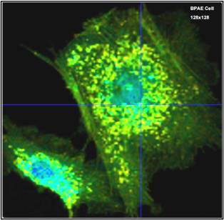
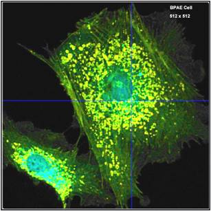
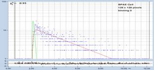
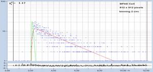
Fig. 29: Effect of spatial binning. Left: 128 x 128 pixels, no
binning , Right: 512 x 512 pixels, binning of
5x5 pixels
De-Convolution
In a real FLIM system the fluorescence is
excited by laser pulses of non-zero width, and detected by a detector with a
temporal response of non-zero width. The effect on the temporal shape of the
recorded signal is shown graphically in Fig. 30. The laser pulse is thought to
be broken down into a sequence of (infinitely) narrow pulses of different
amplitude (Fig. 30, left). Each of these sub-pulses produces a fluorescence
decay of an amplitude proportional to the amplitude of the sub-pulse, and
starting at the time of the sub-pulse. The sum of all these decay functions is
the real optical waveform of the fluorescence signal, see bottom of Fig. 30,
left. The real fluorescence signal is measured by a detector the temporal
response of which has non-zero width, see Fig. 30, middle. Again, the detector
response can be thought to consist of a sequence of infinitely short pulses.
Also here, the measured waveform is the sum of shifted signal components of
different amplitude.
Fig. 30: Left: Convolution of the laser pulse with the fluorescence decay.
Middle: Convolution of the real fluorescence waveform with the detector
response. Right: Laser pulse and detector response combined into IRF pulse,
convolution of fluorescence decay with IRF.
The transformation of the signal waveforms
shown above is called convolution. Mathematically, the signal transformation
is described by the commonly known 'convolution integral' [1]. The laser pulse
shape and the detector response can be combined in a single instrument
response function, or IRF, see Fig. 30, right. The IRF is the convolution of
the laser pulse shape with the detector response, i.e. the pulse shape the
system would record if it directly detected the laser. The convolution of the
fluorescence decay function with this IRF delivers the same result as the two
subsequent convolution steps shown in Fig. 30, left and middle.
The convolution integral cannot be
reversed, i.e. there is no analytical expression of f(t) for a given fm(t)
and IRF(t) [1]. The standard approach to solve the de-convolution
problem is to use a fit procedure: A model function of the fluorescence decay
function is defined, the convolution integral of the model function and the IRF
is calculated, and the result is compared to the measured data. Then the
parameters of the model function are varied until the best fit with the
measured data is obtained. This operation is performed for all pixels if the
image.
Weighted Least-Square Fit
The principle of the traditional weighted least-square
(WLS) fit is shown in Fig. 31. The differences, delta(t), between the points of
the model function, fmod(t), and the data points, n(t), are calculated.
In principle, the squares of the differences, delta(t)2, could be
calculated, summed up, and this sum be used as an optimisation parameter.
Fig. 31:
Least-square fit
For fluorescence decay curves, this
procedure has a flaw. The photon numbers, n(t), are Poisson-distributed. That
means the noise is larger in channels with higher photon number: The noise in n(t)
is n(t)1/2 [1, 12]. Therefore, the squares of the differences
must be weighted with the reciprocal of the expected value of the noise.
The required weighting of the delta-squares
is the problem of the least-square fit. The correct weight according to the Poisson
distribution would be 1/n(t). This is, of course, not possible because
there are time channels with n(t)=0. The weight of these channels would
be infinite, which is a practical impossibility. The commonly used solution is
to use a weight of 1/(n(t)+1):

The weighting with 1/n(t)+1 avoids
the singularity problem for n(t)=0, but, of course, does not weight the
deltas in channels with low n(t) or n(t)=0 correctly. The result
is a bias towards shorter lifetimes for decay data of low photon number.
Maximum-Likelihood Fit
Unlike previous SPCImage versions,
SPCImage NG uses a maximum-likelihood algorithm (or maximum-likelihood
estimation, MLE) for fitting the data. In contrast to the usual least-square
fit, the MLE algorithm takes into account the Poissonian distribution of the
photon numbers. Compared to the least-square method, the fit accuracy is
improved especially for low photon numbers, and there is no bias toward shorter
lifetime as it is observed for the least-square fit. The maximum-likelihood fit
is based on calculating the probability that the values of the model function
correctly represent the data points of the decay function. The principle is
illustrated in Fig. 32. To each point of the model function, fmod(t),
a Poissonian distribution,

with an expectation value equal to E=fmod(t),
is associated, Fig. 32, right. From this distribution, the probability, p(n(t)),
is calculated, that a data point with the photon number, n(t), appears
in the corresponding time channel of the measurement data. The probability, p(n(t)),
is a measure of how likely it is that the point of the model function is a
correct representation of the data. p(n(t)) is calculated for all time
channels, i.e. for all pairs of data points and model-function points. The product
of these probabilities is the probability that the model function represents
the data. The parameters of the model functions are then optimised until the
maximum product of the probabilities is obtained.
Fig. 32: Principle of MLE fit. For each point of the model function, fmod(t),
a Poissonian distribution is associated. The function delivers a probability
p(n(t)), that a given data point, n(t) fits to the corresponding point of the
model function. The product of p(n(t)) over all time channels is used for
optimising the parameters of the model function.
The MLE fit has no problem with data points
with low photon number or even with a photon number of zero. The Poissonian
distribution associates correct probabilities to all these situations, and the
product of these probabilities correctly describes the quality of the fit. Consequently,
there is no bias toward shorter lifetime, as it occurs in the weighted least
square fit.
For comparison with older data sets the
weighted least-square fit and the first-moment lifetime calculation are still
available in SPCImage NG. The analysis method is selected in the 'Model' panel,
see Fig. 33. MLE can (and should) be declared the default under 'Preferences',
Other Settings'. The least-square fit and the first-moment lifetime calculation
are not running GPU processing.
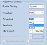

Fig. 33: Selecting MLE under Model, Algorithmic Setting (left) and
declaring MLE the default method under Preferences, Other Settings.
Principle of Phasor Analysis
SPCImage FLIM analysis software combines
time-domain multi-exponential decay analysis with phasor analysis. Phasor
analysis expresses the decay data in the individual pixels as phase and
amplitude values of a periodic waveform in a polar diagram, or the 'Phasor
Plot' [15]. The principle is illustrated in Fig. 34.

Fig. 34:
Principle of phasor analysis
Independently of their location in the
image, pixels with similar decay signature form clusters in the phasor plot. Different
phasor clusters can be selected, and the corresponding pixels back-annotated in
the time-domain FLIM images, see Fig. 35 and Fig. 36. Moreover, the decay
functions of the pixels within the selected phasor range can be combined into a
single decay curve of high photon number. This curve can be analysed at high
accuracy, revealing decay components that are not visible by normal pixel-by-pixel
analysis, see Fig. 36. Please see [1], 'The bh TCSPC Handbook', chapter
'SPCImage Data Analysis'.
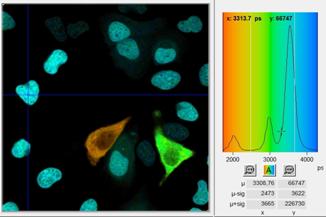
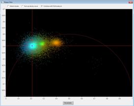
Fig. 35: Left: Lifetime image and lifetime histogram. Right: Phasor plot.
The clusters in the phasor plot represent pixels of different lifetime in the
lifetime image. Recorded by bh Simple-Tau 152 FLIM system with Zeiss LSM 880.
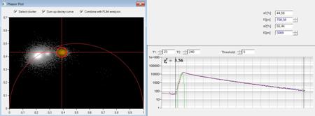
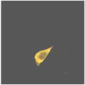
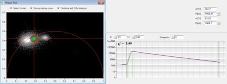
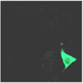
Fig. 36: Left: Selecting two different clusters in the phasor plot. Middle:
Combination of the decay data of the corresponding pixels in a single decay
curve. Right: Display of the pixels corresponding to the selected cluster in
the phasor plot.
IRF Definition
In a laser scanning system it is difficult,
if not impossible, to measure an IRF. The excitation wavelength is usually
blocked by filters, and a fluorophore with sufficiently short lifetime is not
available. In multiphoton microscopes recording of an SHG signal is an option,
but also this is not free of pitfalls. The SHG is emitted in forward direction
and only partially scattered back into the detection beam path. This can
broaden the recorded signal or distort it by reflections from the condenser
lens or other elements in the transmission path of the microscope. SPCImage
therefore provides several ways to avoid IRF recording altogether.
Auto IRF from FLIM data
An IRF is calculated from the rising edge
of the fluorescence decay curves in the FLIM data. The calculation is run on
the combined data of several pixels around the brightest spot in the image. The
IRF obtained this way is reasonably correct when the recorded signal is
fluorescence with a lifetime several times longer than the width of the IRF.
Systematic deviations may occur when SHG or an extremely fast fluorescence
decay component are present, or when the rising edge is distorted by laser
leakage. Nevertheless, the 'Auto IRF' works well [1], and has been used
successfully since the introduction of the first SPCImage version in 2000.
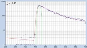
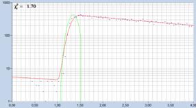
Fig.
37: Auto IRFs (green curves) calculated from FLIM data
Rectangular IRF
A rectangular IRF can be defined manually.
It is used preferentially for PLIM analysis. Excitation of PLIM occurs over the
on-time of the laser in the PLIM modulation period. The effective IRF can thus
be modelled by a rectangle [13].
Synthetic IRF of the type x·e-x
A function of the type x·e-x closely
resembles the IRF of hybrid detectors with GaAsP cathodes [1]. It also fits
reasonably well to the response of many other detectors. SPCImage NG provides a
function to automatically adjust the parameter x to the shape of the effective
IRF. For lasers with pulse width above 1 ps the detector IRF can be
convoluted with a Gaussian function of selectable width. The definitions are
shown in Fig. 38, two examples for IRFs of the x·e-x type and the
fit of fluorescence data with them are shown in Fig. 39.
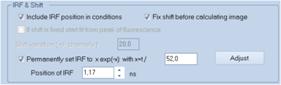
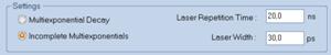
Fig. 38:
Definitions for IRF of the type x·e-x
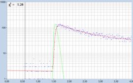
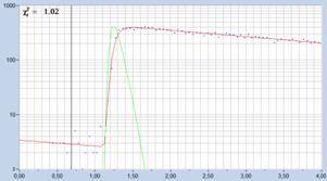
Fig. 39: IRF
of the type xe-x. Left: Modelled for ps diode laser plus HPM-100-06
hybrid detector. Right: IRF modelled for HPM-100-40 hybrid detector and ps
diode laser.
The synthetic IRF works even for FLIM data
with an extremely fast decay component. Fig. 40 shows mushroom spores with a
dominating decay component on the order of 24 ps. The figure shows that a
reasonable fit is obtained even for the fast peak of the decay curve.
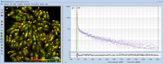
Fig. 40: Spores of Boletus edulis, analysed with a synthetic IRF.
The amplitude-weighted lifetime is 30 ps, the lifetime of the fast
component is about 24 ps. Two-photon FLIM, HPM-100-06 Ultra-fast detector,
SPC-150NX TCSPC/FLIM module.
IRF from recorded data
For standard FLIM analysis the synthetic
IRF is fully capable of fitting the decay data correctly. Even for data with
extremely fast decay components the synthetic IRF works reasonably well, see
above, Fig. 40. Exceptions are high-resolution experiments where ultra-fast decay
components with lifetimes in the range of the IRF width or shorter are to be
determined. In these cases the synthetic IRF can cause ambiguity, i.e. a
slightly shorter IRF width and slightly longer fast-component lifetime and vice
versa can yield the same fit quality.
Ultra-fast-decay FLIM is normally performed
with femtosecond excitation and two-photon excitation. Under these conditions
an IRF is best obtained from SHG data. An image is recorded with the same TCSPC
parameters as the FLIM data to be analysed. A suitable area in this image is
selected, and the curve within this area is declared an IRF. Please see [1] for
details. An IRF recorded from finely ground sugar is shown in Fig. 41. For data
analysis with this IRF please see Fig. 16, page 11 of this brochure.
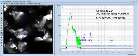
Fig. 41: IRF
from SHG of powdered sugar. Ultra-high resolution, 300 femtoseconds / channel
In multiphoton FLIM the IRF can sometimes
be obtained from the FLIM data themselves. These often contain a substantial
amount of SHG signal. Select a region which is dominated by SHG (Fig. 42,
left), declare the waveform of this area an IRF (Fig. 42, middle), and run the
data analysis with this IRF (Fig. 42, right).
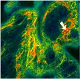
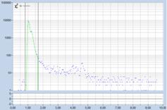
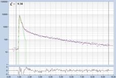
Fig. 42: IRF from multiphoton tissue FLIM data. Find a region dominated by
SHG, declare the signal of this region an IRF, and analyse the image with it.
Model Functions
Sum of Exponentials
The fluorescence decay function obtained
from a homogeneous population of molecules in the same environment is a single
exponential. Decay functions of mixtures of different molecules or of molecules
in inhomogeneous environment are sums of exponential functions of different
decay time. The basic model functions used in SPCImage are therefore sums of
exponential terms:
Single-exponential model: 
Double-exponential model: 
Triple-exponential model: 
The models are characterised by the
lifetimes of the exponential components, t, and the amplitudes of
the exponential components, a. In principle, models with any number of
exponential components can be defined. However, higher-order models become so
similar in curve shape that the amplitudes and lifetimes cannot be obtained at
any reasonable certainty. Therefore, FLIM analysis does not use model functions
with more than three components. A typical example is shown in Fig. 43. The
single exponential model does not fit the data. The double-exponential model
fits well, the triple-exponential reveals a weak third component of long
lifetime.
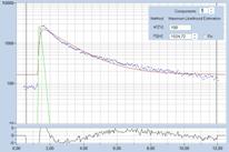
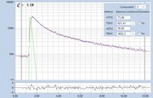
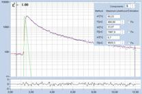
Fig. 43: Fit
of decay data with a single, double, and triple-exponential model.
Incomplete Decay Model
At high laser repetition rate the residual fluorescence
from the previous laser pulses cannot be ignored. SPCImage has an 'Incomplete
Decay' model which takes the residual fluorescence into account. Fig. 44 and Fig.
45 give a comparison of the ordinary multi-exponential model (left) and the
incomplete-decay model (right). The ordinary model interprets the intensity
left of the rising edge of the decay curve as offset, the incomplete-decay
model fits it correctly with fluorescence from the previous pulses. For a fluorescence
decay of 2.3 ns and 80 MHz repetition rate the difference between the two
models is still small, see Fig. 44. However, for a lifetime of 4 ns the
difference is already 14%, an error which cannot be tolerated. Please see Fig. 45,
right.
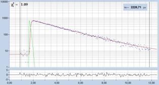
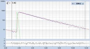
Fig. 44: Fit of the fluorescence decay of a Calcium sensor, lifetime
2.29 ns, excitation with Ti:Sa laser at 80 MHz. Left: ordinary
double-exponential model. Right: Incomplete decay model.
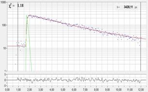
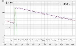
Fig. 45: Fit of the fluorescence decay of fluorescein, lifetime
4.0 ns, excited at 80 MHz. The difference between the models is 14%.
The incomplete-decay model makes it
possible to record FLIM with fluorophores of more than 5 ns with
multiphoton microscopes without the need of reducing the laser repetition rate.
Another example is shown in Fig. 46.
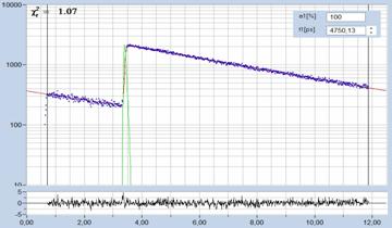
Fig. 46:
Fluorescence decay of a 4.75 ns dye recorded in a two-photon microscope.
Laser repetition rate 80 MHz.
Shifted-Component Model
In clinical FLIM it happens that one or
several decay components are shifted in time. A typical example is ophthalmic
FLIM (FLIO) where fluorescence from the lens of the eye interferes with
fluorescence of the fundus. The lens fluorescence appears about 150 ps
before the fundus fluorescence. The shifted-component model takes this shift
into account [14].
A demonstration is given in Fig. 47 and Fig.
48. A FLIO decay curve together with the model definition is shown in Fig. 47. A
triple-exponential model is used; the lens component is modelled by the third
decay component and shifted 150 ps towards earlier times. As a result, the
model fits the lens component correctly, including the kink in the rising edge
caused by the early arrival of the lens fluorescence.
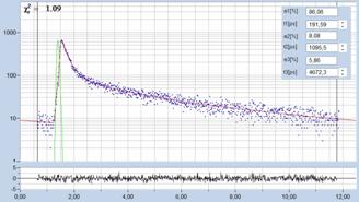
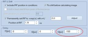
Fig. 47: Decay curve from FLIO data. Fit with shifted-component model, third
decay component shifted by 150 ps to earlier time.
FLIO lifetime images obtained by the
ordinary multi-exponential model and by the shifted-component model are compared
in Fig. 48. For the ordinary model, the lens fluorescence causes a substantial
shift of the mean lifetime, tm, to longer values. The shifted-component model is
able to deliver an image which contains only the fundus fluorescence, modelled
by the components t1 and t2. The corresponding image of the lifetime tm12 is
shown in Fig. 48, right. It shows the correct lifetime of the fundus of the eye
[14].
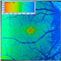
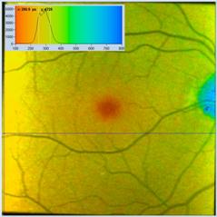
Fig. 48: Comparison of FLIO analysis with the ordinary 3-component model
(left) and with the shifted-component model (right). Due to the contribution of
the lens fluorescence, the ordinary image is biased towards long lifetime. The delayed-component model delivers an image that does not contain the lens fluorescence, showing
the correct lifetime of the fundus of the eye.
Summary
With the new SPCImage NG version bh's TCSPC FLIM data analysis software obtained a substantial upgrade. Obvious features are a
smooth combination of phasor analysis with time-domain analysis, accuracy
improvement by MLE analysis, and speed enhancement by GPU processing. Other
functions, such as improved modelling of the IRF, improved decay models, and
the ability to display additional combinations of multi-exponential-decay
parameters further enhance he performance of SPCImage. New applications can be
expected especially in the fields of live cell imaging, clinical FLIM,
metabolic FLIM, ultra-fast FLIM, and FLIM of dynamic processes in live systems.
References
1.
W. Becker, The bh TCSPC handbook. Becker &
Hickl GmbH, available on www.becker-hickl.com
2.
Becker & Hickl GmbH, The HPM‑100-40
hybrid detector. Application note, available on www.becker-hickl.com
3.
Becker & Hickl GmbH, Sub-20ps IRF Width from
Hybrid Detectors and MCP-PMTs. Application note, available on
www.becker-hickl.com
4.
W. Becker, V. Shcheslavskiy, A. Bergmann, FLIM
at a Time-Channel Width of 300 Femtoseconds. Application note, available on
www.becker-hickl.com
5.
W. Becker, C. Junghans, A. Bergmann, Two-Photon
FLIM of Mushroom Spores Reveals Ultra-Fast Decay Component. Application note
(2021), available on www.becker-hickl.com
6.
W. Becker, T. Saeb-Gilani, C. Junghans, Two-Photon
FLIM of Pollen Grains Reveals Ultra-Fast Decay Component. Application note
(2021), available on www.becker-hickl.com
7.
Becker & Hickl GmbH, Two-Photon FLIM with a
Femtosecond Fibre Laser. Application note, available on www.becker-hickl.com
8.
Becker & Hickl GmbH, Precision
Fluorescence-Lifetime Imaging of a Moving Object. Application note, available
on www.becker-hickl.com
9.
W. Becker, A. Bergmann, L. Braun, Metabolic
Imaging with the DCS-120 Confocal FLIM System: Simultaneous FLIM of NAD(P)H and
FAD, Application note, available on www.becker-hickl.com (2018)
10.
W. Becker, R. Suarez-Ibarrola, A. Miernik, L. Braun,
Metabolic Imaging by Simultaneous FLIM of NAD(P)H and FAD. Current Directions
in Biomedical Engineering 5(1), 1-3 (2019)
11.
W. Becker, A. Bergmann, M. Schubert, S.
Smietana, Lifetime-Intensity Mode Delivers Better FLIM Images. Application
note, available on www.becker-hickl.com
12.
W. Becker, Bigger and better photons. The road
to great FLIM results. Education brochure, available on www.becker-hickl.com
13.
Becker & Hickl GmbH, Simultaneous
Phosphorescence and Fluorescence Lifetime Imaging by Multi-Dimensional TCSPC
and Multi-Pulse Excitation. Application note, available on www.becker-hickl.com
14.
W. Becker, A. Bergmann, L. Sauer,
Shifted-Component Model Improves FLIO Data Analysis. Application note, Becker
& Hickl GmbH (2019)
15.
M. A. Digman, V. R. Caiolfa, M. Zamai, and E. Gratton, The phasor approach to fluorescence
lifetime imaging analysis, Biophys J 94, L14-L16 (2008)
Contact:
Wolfgang Becker
Becker & Hickl GmbH
Berlin, Germany
becker&becker-hickl.com
www.becker-hickl.com