Megapixel FLIM with bh TCSPC Modules
The New SPCM 64-bit
Software
Wolfgang Becker, Stefan Smietana, Axel Bergmann,
Becker & Hickl GmbH, Berlin, Germany
Abstract: Becker & Hickl have recently
introduced version 9.60 of their SPCM TCSPC data acquisition software. SPCM
version 9.60 not only runs on 64‑bit computers, it is a real 64-bit
application. It thus takes full advantage of the capabilities of 64-bit
Windows. The most significant one is that a large amount of memory can be
addressed. As a result, FLIM data can be recorded with unprecedented numbers of
pixels and time channels. Moreover, the large memory
space allows multi-dimensional FLIM procedures to be used without compromising
spatial resolution. Multi-spectral FLIM can be recorded at unprecedented spatial
resolution, the image area can be increased by spatial mosaic recording, Z
stacks can be efficiently acquired without the need of intermediate data save
actions, and fast time series of FLIM data can be accumulated. This application note gives an overview of
the performance that can be achieved by running bh TCSPC FLIM modules with the
new software.
Image Size in FLIM
TCSPC FLIM has been introduced in 1996 with
the SPC-535 modules of Becker & Hickl. The first applications were in ophthalmology,
where FLIM was shown to detect early stages of eye diseases. FLIM for laser
scanning microscopy was introduced with the SPC-730 modules in 1998. The FLIM
data were built up by the on-board processing logics in the memory of the TCSPC
module. The size of the FLIM images was therefore limited by the size of the
on-board memory. Typical images had 128 x 128 pixels, and 256 time
channels per pixel. The image size increased by a factor of four with the introduction
of the SPC‑830 modules. The data format typically used by these modules was
256 x 256 pixels, and 256 time channels [1, 2].
A possible way to record larger images is
to transfer the data into the computer photon by photon, and build up the FLIM data
in the memory of the computer. A suitable operation mode, the FIFO Mode [1, 2], had been implemented in bh SPC modules
already in 1996. However, the bus transfer speed and the processing capabilities
of the PCs of the 1990s was insufficient for this kind of operation. At count
rates above 100 kHz, as they are routinely used in FLIM, the computer was not
able to read the single-photon data from the SPC module and simultaneously
process them to build up a photon distribution.
The situation changed with the introduction
of multi-core PCs. The tasks of data transfer and data processing could now be
shared between the CPU cores. Count rate in the FIFO mode was no longer a
problem. bh introduced the FIFO Imaging mode for FLIM [6] in 2007. Limited by
the amount of memory addressable by Windows 32 bit, the typical image size was
512 x 512 pixels, 256 time channels. This is more than enough to
obtain diffraction-limited microscopy images of cells and tissue samples at a
time resolution (time-channel width) on the order of a few 10 ps.
However, there are FLIM applications that
make it desireable to record FLIM data of larger size. Examples are imaging of
a large number of cells in the same field of view, or FLIM measurements over
additional parameters, such as wavelength, depth in the sample, or time after a
stimulation. Such application require an amount of memory space which is only
available in a 64-bit environment.
FIFO Imaging with Windows 64 bit
A typical PC running Windows 64 bit is
able to use about 16 GB of memory, as compared to 4 GB for Windows 32 bit.
bh therrfore released a 64-bit version of the SPCM data acquisition software. Provided
the computer has enough memory SPCM 64 bit can record images as large
as 2048 x 2048 pixels and 256 time channels, or 1024 x 1024
pixels and 1024 time channels. Several such data sets can be recorded
simultaneously if the FLIM system has several TCSPC channels.
SPC system parameters for an image of
2048 x 2048 pixels and 256 time channels are shown in Fig. 1. Of
course, the scan format of the scanner must be at least of the same size [4, 5].
Settings for the bh DCS‑120 confocal scanner are shown on the right.
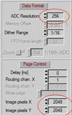
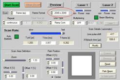
Fig. 1: Image format definitions for an image of 2048 x 2048
pixels and 256 time channels. Left: SPCM system parameters, Data Format and
Page Control section. Right: DCS‑120 scanner control panel.
An image of a convallaria sample recorded
with these parameters is shown in Fig. 2. The image on the left is the entire
FLIM image, the image on the right is a digital zoom into the area marked in
the in the image shown left.
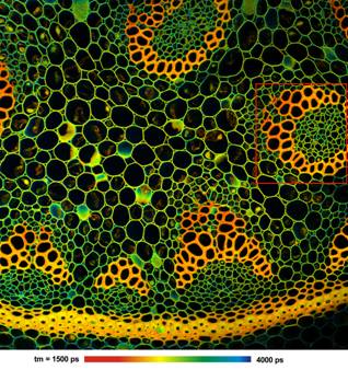
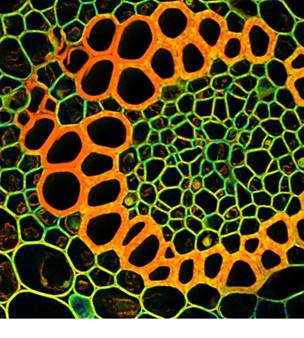
Fig. 2: FLIM recorded with 2048 x 2048 pixels and 256 time
channels. Left: Entire image. Right: Digital zoom into indicated area of left
image. bh DCS‑120 confocal scanning FLIM system, Zeiss Axio Observer
microscope, x20 NA=0.5 air lens.
FIFO imaging with the 64-bit SPCM software
becomes especially powerful when several images are to be recorded
simultaneously. Fig. 3 shows images recorded by a dual-channel parallel TCSPC (SPC‑152)
system. The sample was a BPAE cell labelled with Alexa 488 and Mito Tracker.
The excitation wavelength was 473 nm. The images were recorded
simultaneously in two wavelength intervals, from 484 nm to 560 nm,
and 560 nm to 700 nm. The FLIM data format for both images is 1024 x 1024
pixels and 1024 time channels. The total size of the FLIM data set is 4 GB. A
decay curve at a selected pixel position is shown in Fig. 4.
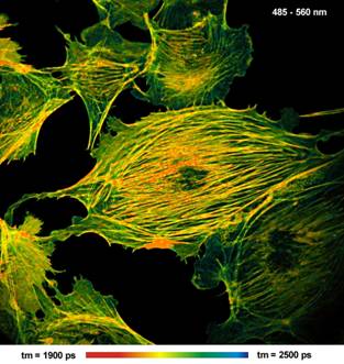
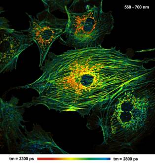
Fig. 3: Dual-channel parallel FLIM with two bh SPC 150 TCSPC modules.
Both images, each with 1024 x 1024 pixels and 1024 time channels, were
recorded simultaneously. bh DCS-120 confocal scanning system with Zeiss Axio
Observer microscope, x63 NA=1.3 oil immersion lens.
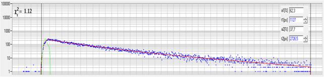
Fig. 4: Fluorescence decay function at selected position of Fig. 3, left.
The decay function is recorded in 1024 time channels. Blue dots: Photon numbers
in the time channels. Red curve: Fit with a double-exponential model.
The large data formats provided by SPCM 64
bit are also desirable for multi-wavelength FLIM recordings. With Windows 32
bit, the maximum data format for the MW-FLIM 16-channel multi-wavelength
detector was limited to 256 x 256 pixels, 64 time channels, or
128 x 128 pixels, 256 time channels. With Windows 64 bit
and SPCM V 9.60 images with 512 x 512 pixels and 256 time
channels can be obtained. This is 16 times the number of pixels obtained with
Windows 32 bit.
Fig. 5 shows a multi-wavelength FLIM
recording of a Convallaria sample. The data were recorded by a bh DCS‑120
confocal scanning system with a bh MW-FLIM GaAsP 16-channel detector. 16 lifetime
images in 16 wavelength intervals were recorded simultaneously. The data
were recorded at a resolution of 512 x 512 pixels and 256 time
channels per pixel. The wavelength channel width was 12.5 nm, the centre
wavelengths of the channels range from 490 nm to 690 nm. The size of
the entire multi-wavelength data set is 2 GB.
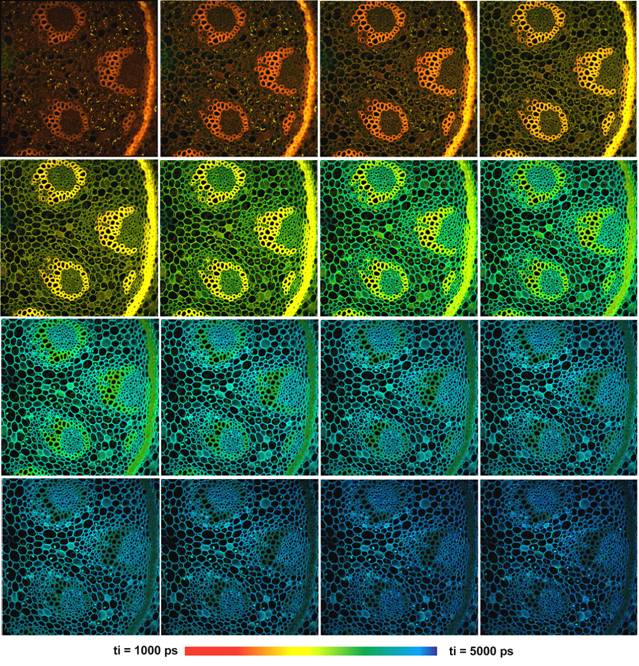
Fig. 5: Multi-wavelength FLIM with a bh MW-FLIM GaAsP 16-channel detector.
16 images with 512 x 512 pixels and 256 time channels were recorded
simultaneously. Wavelength from upper left to lower right, 490 nm to 690 nm,
12.5 nm per image. DCS‑120 confocal scanner, Zeiss Axio Observer
microscope, x20 NA=0.5 air lens.
Fig. 6 demonstrates the true spatial resolution
of the data. Images from two wavelength channels, 502 nm and 565 nm, of
the data shown Fig. 5 are displayed at larger scale and with individually
adjusted lifetime ranges. The spatial resolution is comparable with what
previously could be reached for FLIM at a single wavelength. Nevertheless, the
decay data are recorded at a temporal resolution of 256 time channels. Decay
curves for selected pixels of the images are shown in Fig. 7.
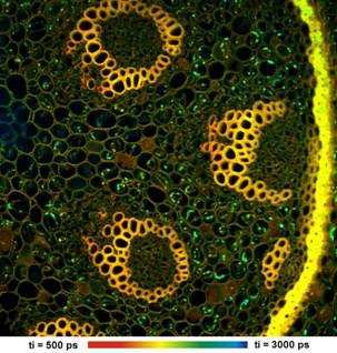
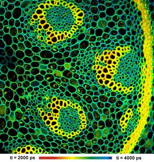
Fig. 6: Two images from the array shown in Fig. 5, displayed in larger
scale and with individually adjusted lifetime range. Wavelength channels 502 nm
(left) and 565 nm (right). The images have 512 x 512 pixels and
256 time channels.
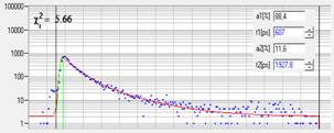
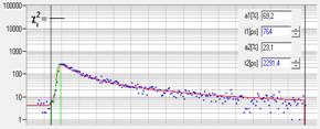
Fig. 7: Decay curves at selected pixel position in the images shown above.
Blue dots: Photon numbers in the time channels. Red curve: Fit with a
double-exponential model.
Mosaic FLIM
To record images larger than the maximum
field diameter of the microscope lens laser scanning microscopes use a tile
imaging function. The microscope scans an image at one position of the sample,
then offsets the sample by the size of the scan area, and scans a new image.
The process is repeated, and the images of the individual frames are stitched
together. This way, a sample area larger than the field of view of the
microscope lens can be imaged.
X-Y Mosaic
The large memory size available in the 64
bit environment allows tile imaging to be combined with FLIM. In the memory of
FLIM system, a two-dimensional mosaic of FLIM data blocks is defined. The
number and arrangement of the data blocks is the same as for the tiles in the
imaging procedure of the microscope. The FLIM data structure can thus be
considered one large FLIM image that contains all tiles in the correct
arrangement. Moreover, for each element of the FLIM mosaic a number of frames
is defined which is identical with the number of frames per tile defined in the
microscope. When the microscope starts the scan the FLIM system starts to
record an image in the first mosaic element. It continues to do so until the
defined number of frames has been completed, and then switches to the next
mosaic element. This way, the FLIM system switches through all mosaic elements,
filling all of them with data of the corresponding tiles. The procedure ends
when the microscope has completed the last frame of the last tile.
An example of a Mosaic FLIM is shown in Fig.
8. The image was recorded by a Zeiss LSM 710 Intune (tuneable excitation)
system in combination with a bh Simple-Tau 150 FLIM system. The mosaic has
4x4 elements, each element has 512 x 512 pixels with 256 time channels. The
complete mosaic has thus 2048 x 2048 pixels, each pixel holding 256
time channels. The sample area covered by the mosaic is 2.5 mm x
2.5 mm.
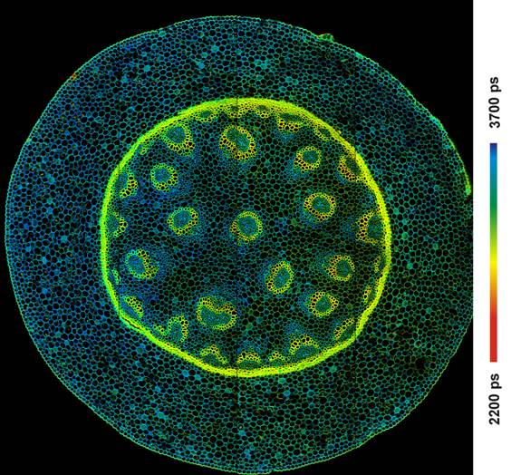
Fig. 8: Mosaic FLIM of a Convallaria sample. The mosaic has 4x4 elements,
each element has 512x512 pixels, each pixel has 256 time channels. Zeiss
LSM 710 Intune system with bh Simple-Tau 150 FLIM system.
Mosaic FLIM for Z-Stack recording
The same FLIM procedure can be used to
record z-stacks of FLIM images. The number of mosaic elements is made identical
with the number of z planes the microscope scans. The number of frames per
mosaic element is selected according to the number of frames per z plane.
Compared with a z-stack FLIM procedure by a record-and-save sequence [2, 7] mosaic
FLIM has the advantage that the synchronisation between the microscope and the
FLIM system is easier, and no time has to be reserved for the saving actions.
Moreover, the data of all z planes are recorded in one and the same photon
distribution. The data analysis can therefore be run for the data of all z
planes together. This makes it easier to maintain exactly the same fit
conditions and model parameters for all z planes, and to extract global
parameters form the entire array. An example is shown in Fig. 9.
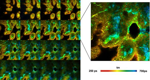
Fig. 9: Z-stack recorded by Mosaic FLIM. Pig skin stained with Indocyanin
Green. Zeiss LSM 7 MP OPO system, 16 planes from 0 to 60 µm from top of
sample, each plane 512x512 pixels, 256 time channels. Amplitude-weighted
lifetime of double-exponential decay.
Temporal Mosaic FLIM
The usual way to record time series by FLIM
is to record a sequence of images and save the subsequent images in consecutive
files [1, 2, 4, 5]. Mosaic FLIM
provides a second way to record time series. In that case, every element of the
mosaic represents one step of the series. Each element can be a single frame or
a defined number of frames of the scan.
An example is shown in Fig. 10. The sample
was a fresh moss leaf, the microscope a bh DCS-120 confocal FLIM system [4]. The time runs from lower left to upper
right. The excitation light causes a non-photochemical transient in the
chlorophyll fluorescence [8], resulting in a decrease in the fluorescence
lifetime over the time of exposure.
Fig. 10: Time series recorded by mosaic imaging. Non-photochemical
transients in chloroplasts of a moss leaf. 64 mosaic elements for consecutive
times after turn-on of excitation light. Acquisition time per element 1 second,
total time of sequence 64 seconds, image size of each element 128 x 128 pixels,
256 time channels. Time runs from lower left to upper right. bh DCS-120
confocal FLIM system with SPC-150 TCSPC modules, SPCImage data analysis
software.
Mosaic time series recording has two
advantages over the conventional record-and-save procedure. First, the
transition from one mosaic element to the next occurs instantaneously. There
are no time gaps between the steps of the sequence. Therefore, very fast time
series can be recorded.
The biggest advantage is, however, that mosaic
time series data can be accumulated: A sample would be repeatedly stimulated by
an external event, and the start of the mosaic recording be triggered by the
stimulation. With every new stimulation the recording procedure runs through
all elements of the mosaic, and accumulates the photons. Accumulation allows
data to be recorded without the need of trading photon number and lifetime
accuracy against the speed of the time series. Consequently, the time per step
(or mosaic element) is only limited by the minimum frame time of the scanner.
For pixel numbers on the order of 128x128 pixels and small scan areas
galvanometer scanners reach frame times on the order of 50 milliseconds.
Resonance scanner are even faster. This brings the time-series resolution into
the range where even lifetime changes induced by Ca2+ transients in
neurons can be recorded. Previously, this was only possible by FLITS, i.e.
recording the decay functions within the pixels of a line scan [3].
Fig. 11 shows a mosaic FLIM recording of
the Ca2+ transient in cultured neurons after stimulation with an
electrical signal. Oregon Green was used as a Calcium sensor. A Zeiss LSM
7 MP multiphoton microscope was used to scan the sample. The scan format was
64 x 64 pixels. With 64 x 64 pixels and a zoom factor
of 5, the LSM 7 MP reaches a frame time of 38 ms. The FLIM data were
recorded by a bh SPC‑150 module. A FLIM mosaic size of 8 x 8 elements
was defined. The stimulation period was 3 seconds. 150 milliseconds before
every stimulation a recording through the entire 64-element mosaic was started.
With the frame time of 38 ms, the acquisition thus runs through the entire
mosaic in 2.43 seconds. 100 such acquisition runs were accumulated. The result
shows clearly the increase of the fluorescence lifetime of the Ca2+
sensor in the mosaic elements 4 to 6, and a return to the resting state over
the next 10 to 15 mosaic elements (380 to 570 ms).
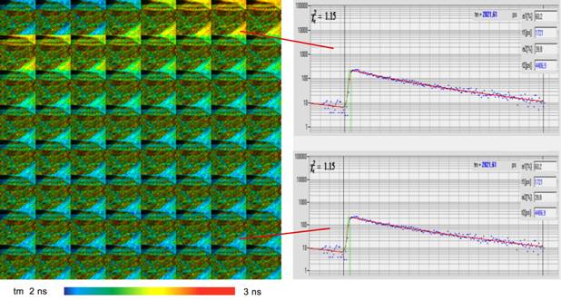
Fig. 11: Temporal mosaic FLIM of the Ca2+
transient in cultured neurons after stimulation with an electrical signal. The
time per mosaic element is 38 milliseconds, the entire mosaic covers 2.43
seconds. Experiment time runs from upper left to lower right. Photons were
accumulated over 100 stimulation periods. Recorded by Zeiss LSM 7 MP and bh SPC‑150
TCSPC module. Data courtesy of Inna Slutsky and Samuel Frere, Tel Aviv University,
Sackler Faculty of Medicine.
Data Acquisition and Data Analysis Times
Acquisition times for megapixel FLIM data
are naturally long. To obtain a given signal-to-noise ratio, a
1024 x 1024 pixel image needs 16 times the photons of a
256 x 256 pixel image. Assuming that the 256 x 256 image is
recorded in 30 seconds the 1024 x 1024 image would need 8 minutes of
acquisition time to obtain the same number of photons per pixel and the same
lifetime accuracy. Fortunately, in practice the acquisition time often does not
scale linearly with the pixel number. The reason is that images with large
pixel numbers are usually over-sampled. Under these conditions, the lifetime
data in adjacent pixels (i.e. the pixels within the Airy-disc diameter) are
highly correlated. It is then possible to use pixel binning for the lifetime
data in the SPCImage data analysis. The photon number per pixel required for a
given lifetime accuracy is than much smaller. Please see chapters on data
analysis in [2], [4], or [5].
Data analysis times for large FLIM data
sets can be long as well. Note that a 1024 x 1024 image with 1024
time channels is actually a stack of 1024 one-megapixel images! Because the
analysis procedure has to run through all pixels and time channels the
processing time scales linearly with the numbers of pixels and time-channels.
To speed up the data analysis we recommend to select Multi-Thread Processing
in the Options section. Please also make sure that you do not analyse the
data with conflicting parameters: For instance, fitting a data set with a
multi-exponential model and a free Shift parameter causes a conflict between
a possible change in a fast decay component and a change in the shift. The data
analysis time then increases dramatically.
Before starting the final analysis of a
large image, we recommend to analyse a small region of interest, and set
appropriate model parameters. The final analysis will then run smoothly, and
need not be done twice. For a fast preview of the lifetimes, we recommend to
use the Moments analysis of SPCImage, see Options, Model.
Please note that recent SPCImage versions
have a Batch Processing function [2]. It is used to analyse several FLIM data
sets with the same model and fit parameters. Once the process has been started,
batch processing does not require user interaction. Several megapixel FLIM data
sets can then be analysed over night.
Conclusion
The bh FLIM systems with version 9.6 SPCM
64 bit software or later are able to record images of unprecedented
numbers of pixels and time channels. One may argue that these pixel numbers are
far beyond the number required to resolve a single cell at reasonable spatial oversampling.
This is certainly correct. There are, however, FLIM applications that make it
desirable to scan much larger fields of view than the one filled by a single
cell. A typical case is when the fluorescence-decay signature of a large number
of cells is to be compared. Being able to record many cells in the same field
of view is then a clear advantage. A large field of view is also an advantage
for tissue imaging. The pixel numbers obtained by the new software are on the
same order as the maximum useful pixel numbers for the best microscope lenses
when these are used at their maximum field of view. Another advantage of the
large memory space available by SPCM 64 bit is that FLIM data with additional
dimensions can be recorded without compromising spatial resolution. This allows
the user to record multi-spectral FLIM at unprecedented spatial resolution, to
increase the image area by spatial mosaic recording, and to efficiently acquire
Z stacks and fast time series of FLIM data.
Compatibility
The FIFO imaging mode in the 64 bit
version of the SPCM software can be used for all FLIM systems based on the bh
SPC‑150, SPC‑152, and SPC-154 TCSPC modules, the
Simple-Tau 150, 152, and 154 systems, similar SPC‑160-based systems,
and for SPC‑830-based systems later than May 2007, or serial number
3D0178. The computer used must have 64 bit architecture, and run Windows 7, 64
bit. To take full advantage of the 64 bit capabilities the computer should
be equipped with 16 GB of main memory. Free upgrades of the SPCM software are
available from www.becker-hickl.com.
References
1. W. Becker, Advanced time-correlated single-photon counting techniques. Springer, Berlin, Heidelberg, New York, 2005
2.
W. Becker, The bh TCSPC handbook. Becker &
Hickl GmbH, 5th Edition (2012), www.becker-hickl.com, printed copies available.
3. W. Becker, V. Shcheslavskiy, S. Frere, I. Slutsky, Spatially resolved recording of transient fluorescence
lifetime effects by line-scanning TCSPC. Microsc. Microsc.
Res. Techn. 77, 216-224 (2014)
4.
Becker & Hickl GmbH, DCS-120 Confocal
Scanning FLIM Systems, user handbook. www.becker-hickl.com, printed copies available.
5. Becker & Hickl GmbH, Modular FLIM systems for Zeiss
LSM 510 and 710 family laser scanning microscopes. User handbook.
www.becker-hickl.com, printed copies available.
6. Becker & Hickl GmbH, FLIM in the FIFO Imaging Mode: Large
Images with Small TCSPC Modules. Application note, www.becker-hickl.com
7. Becker & Hickl GmbH, FLIM Systems for Zeiss LSM 710 Record
Z Stacks, Application note, www.becker-hickl.com
8. Govindjee (1995) Sixty-three Years Since Kautsky: Chlorophyll α Fluorescence, Aust. J. Plant
Physiol. 22, 131-160
