We present a lifetime imaging technique that simultaneously records fluorescence and phosphorescence lifetime images in laser scanning systems. It is based on modulating a high-frequency pulsed laser synchronously with the pixel clock of the scanner, and recording the fluorescence and phosphorescence signals by multidimensional TCSPC. Fluorescence is recorded during the on-phase of the laser, phosphorescence during the off-phase. The technique does not require a reduction of the laser pulse repetition rate by a pulse picker, and eliminates the need of using excessively high pulse power for phosphorescence excitation. Laser modulation is achieved either by electrically modulating picosecond diode lasers, or be controlling the lasers via the AOM of a standard confocal or multiphoton laser scanning microscope.

Microsecond Decay FLIM: Combined Fluorescence and Phosphorescence Lifetime Imaging

Wolfgang Becker, Stefan Smietana, Axel Bergmann, Becker & Hickl GmbH

Abstract. We present a lifetime imaging technique that simultaneously records fluorescence and phosphorescence lifetime images in laser scanning systems. It is based on modulating a high-frequency pulsed laser synchronously with the pixel clock of the scanner, and recording the fluorescence and phosphorescence signals by multi-dimensional TCSPC. Fluorescence is recorded during the on-phase of the laser, phosphorescence during the off-phase. The technique does not require a reduction of the laser pulse repetition rate by a pulse picker, and eliminates the need of using excessively high pulse power for phosphorescence excitation. Laser modulation is achieved either by electrically modulating picosecond diode lasers, or be controlling the lasers via the AOM of a standard confocal or multiphoton laser scanning microscope.

Motivation of Using Phosphorescence Decay Imaging

There is a number of radiative relaxation mechanisms which occur on a much longer time scale than fluorescence. The commonly known one is phosphorescence, i.e. emission from the triplet state of organic dyes. Phosphorescence of organic dyes is usually weak at room temperature but can be strong at low temperatures, or if the dyes are embedded in a solid matrix. Strong emission in the microsecond and millisecond range is obtained also for lanthanide complexes [5] and organic complexes of ruthenium [7], platinum [8], and palladium [8]. Of special interest for live-cell imaging is that the luminescence of some of these complexes is strongly quenched by oxygen. The dyes make then excellent oxygen sensors [6, 7, 8, 9, 10]. There are also possible applications as FRET donors [5]. Moreover, slow emission is obtained from a large number of inorganic compounds, quantum dots, nanoparticles, and semiconductors.

Technical Problems of Slow-Decay Imaging

The measurement of long-lifetime luminescence by laser scanning systems faces a number of problems. The first one is related to the excitation of the luminophore. Obviously, the laser pulse period must be longer than the luminescence lifetime. The lifetime for ruthenium is in the lower microsecond range; for europium and terbium dyes it can be in the millisecond range. FLIM with these dyes requires a laser repetition rate no faster than 100 kHz or 100 Hz, respectively. Generating such low repetition rates with pulsed lasers of a laser scanning microscope can be a problem. More important, reduction in repetition rate, for a given pulse power, leads also to a reduction in average excitation power. Attempts to compensate for the drop in average power by higher pulse power are limited by the capabilities of the laser, and by nonlinear effects or even ionisation in the sample. Moreover, any sample that emits phosphorescence necessarily also emits fluorescence. Because fluorescence is fast the peak power of fluorescence becomes very high. This causes transient overload effects in the detectors, preventing the detection of phosphorescence in the first microseconds after the laser pulse. A better way to obtain higher average power is therefore to use longer laser pulse width. Unfortunately, this is not easily possible for most of the lasers. Moreover, long laser pulse width is incompatible with multiphoton excitation.

The second problem is related to scanning. The time the scanner stays within the excited sample volume must be longer than the luminescence lifetime. If the scanner runs off the excited volume within the luminescence decay time photons in the tail of the decay function would be lost, and the recorded decay profile be distorted. Reasonable recording, even of pure intensity images, can thus only be obtained by very slow scanning.

An third problem is aliasing of the laser repetition rate with the pixel frequency: If there are only a few excitation pulses within the pixel time the number of excitation pulses in the pixels varies systematically. This induces Moiré effects in the images. The problem can be solved by synchronising the laser pulses and the pixel frequency, but there is usually no provision for this in a normal laser scanning microscope. Without synchronisation, the pixel time must be at least 100 times longer than the laser period. This leads to unacceptably long frame times.

Of course, the scanner problems can be avoided by using wide-field excitation and detection with a gated camera. However, abandoning scanning also abandons optical sectioning and depth resolution. For most biological applications this is not acceptable.

Modulated Pulsed Laser Operation with TCSPC Recording

The problems described above are avoided by the excitation principle shown in Fig. 1. A high-frequency pulsed laser is used. However, the laser is not run continuously. Instead, it is turned on only for a short period of time, t_on, at the beginning of each pixel [2, 9]. For the rest of the pixel time the laser is turned off. Within the on-time, t_on, the laser excites fluorescence, and builds up phosphorescence. Within the rest of the pixel dwell time, t_off, pure phosphorescence is obtained.

Fig. 1: Principle of Microsecond FLIM

The modulation of the laser is controlled by the bh FLIM system. In the DCS-120 confocal scanning system the laser modulation signal is generated by using the laser-multiplexing features of the bh GVD‑100 scan controller. The BDL‑SMC diode lasers of the DCS‑120 are electronically modulated by applying this signal to their /laseroff inputs [3].

For other microscopes a bh DDG-210 card is added to the FLIM system. The card is triggered by the pixel clock of the microscope and generates the laser modulation signal. Modulation is obtained by combining this signal with the beam blanking signal of the microscope. Laser modulation is then obtained via the acousto-optical modulator of the microscope. The modulation also acts on the Ti:Sa laser of a multiphoton microscope. Thus, microsecond decay imaging becomes applicable also to deep-tissue imaging by two-photon excitation and non-descanned detection.

Lifetime images are built up by using the double-kinetic features of the SPC modules [1, 2]. The principle is shown in Fig. 2. For each photon, the SPC module determines the time, t, within the laser pulse period, and the time, T-T₀, after the modulation pulse. A fluorescence lifetime image is obtained by building up a photon distribution over the micro times, t, of the photons, and the scanner position, x,y, during the T_on periods. The phosphorescence lifetime image is obtained by building up a distribution over the time differences, T-T₀, between the photon times, T, and the laser on pulse edges, T₀. The spatial coordinates come from the scanner position in the moment of the photon detection. Thus, fluorescence and phosphorescence lifetime images are obtained simultaneously, in the same scan, and from photons excited by the same laser pulses.

Multi-wavelength operation is possible by using the routing (or multi-detector) capability of the bh SPC modules [1, 2]. In this case, photons are marked additionally with the wavelength channel in which they were detected. Individual fluorescence and phosphorescence lifetime images are then built up for the individual wavelength channels.

Fig. 2: Simultaneous fluorescence and phosphorescence lifetime imaging. Photon times are determined both with respect to the laser pulse period and with respect to the laser modulation period.

Combined fluorescence / phosphorescence decay imaging has been introduced with the version 9.0 release of the bh SPCM software, April 2010. It is available for SPC‑150 modules and SPC‑830 modules manufactured later than May 20073, or serial numbers later than 3D0178.

TCSPC System Parameter Setup

Typical system setup parameters for the SPC module are shown in Fig. 3. Phosphorescence imaging is obtained by using the MCS (Multichannel Scaler) option in the FIFO Imaging mode. The MCS option is selected in the Configure panel of the System Parameters, see Fig. 3, middle.

The timing reference for MCS imaging comes from the laser modulation. A suitable pulse must be connected to a Marker input at the 15-pin connector of the SPC module [2]. Three marker inputs are available. Trigger defines which of the marker inputs is used as a timing reference. Normally, markers 0, 1, and 2 are used for the pixel clock, line clock, and frame clock from the scanner. The timing reference is then marker 3. However, if the excitation pulses are synchronous with the pixels Trigger can be identical with the pixel clock, i.e. Marker 0. Please make sure that the marker input used for the trigger is enabled in the More Parameters panel of the System Parameters, see Fig. 3 right.

The time channel width (Time per point) of the MCS imaging mode can be any multiples of the macro time clock period. It is defined by a number of Macro Time units. The number of points of the decay curves within the pixels is defined by Points No.. The time range of the curves is given by the product of Time per Point and Points No. It is displayed under Time range. The recorded time interval can be shifted by applying an Offset to the photon times. Both positive and negative offsets are possible.

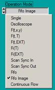
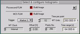
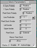
Fig. 3: Definition of MCS FLIM parameters. Left: Operation mode. Middle: Definition of timing parameters and marker selection. Right: Scan format parameters, macro time clock source, and marker enable.

Normally, MCS FLIM recording is performed with the internal macro time clock of the SPC module, see Fig. 3, middle and right. However, for special applications the SYNC frequency can be used. Using the SYNC frequency does, of course, require that the SYNC signal has a constant period, and is present also during the laser off intervals.

To obtain picosecond FLIM (either separately or simultaneously with phosphorescence lifetime imaging) activate the ps FLIM button in the configuration panel. The timing parameters for ps FLIM are selected in the usual way via the TAC parameters of the SPC module [2].

Control of the Laser Modulation

Phosphorescence imaging requires that the excitation laser is on/off modulated by a signal synchronous with the pixel clock, as shown in Fig. 1.

In the Becker & Hickl DCS-120 confocal scanning system [3] pixel-synchronous laser modulation is obtained by using the existing laser-multiplexing features of the scan controller. The DCS system has two ps diode lasers. For phosphorescence lifetime imaging, one laser is used for excitation, the other one is optically turned off. With pixel-synchronous laser multiplexing the modulation scheme shown in Fig. 4, left is achieved.

The setup parameter panel for the DCS‑120 confocal scanner is shown in Fig. 4. Laser Multiplexing is set to Pixel, and a turn-on time for the laser of 12.5% of the pixel time is set. In the Scan Rate definitions the automatic scan rate selection is disabled, and a pixel time a few times longer than the expected phosphorescence decay time is used. Extremely long decay times may require an extension of the available range of the scan rate. This can be obtained by defining a new Max Line Time in the Scan Details panel, see Fig. 4, right.

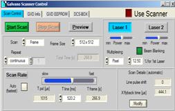
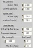
Fig. 4: DCS-120 system, scanner control parameters for phosphorescence decay imaging. Left: definition of laser modulation and scan rate control. Right: Scan Details, definition of maximum line time

For implementation of phosphorescence lifetime imaging in other laser scanning microscopes the microscope must have a pixel clock output from which the laser modulation signal can be derived. Moreover, the microscope must allow for an input of the laser modulation signal to its internal beam blanking. To generate the laser modulation signal we use a Becker & Hickl DDG‑210 programmable pulse generator card. The DDG-210 is triggered by the pixel clock. It delivers a laser modulation signal of programmable width, which is fed back into the beam blanking system of the microscope, see Fig. 5. A second signal is generated to indicate to the TCSPC module whether the laser is on or off. It is used by the TCSPC module to route fluorescence and phosphorescence photons into separate memory blocks [2]. The routing signal is slightly delayed with respect to the modulation signal to account for the delay in the opto-acoustic modulator (AOM) of the microscope.

Fig. 5: On-off modulation of laser in other scanning systems than the DCS‑120. The pixel clock of the microscope triggers the generation of a laser-on pulse in the DDG-210 pulse generator module. The laser-on pulse controls the beam blanking in the microscope. The AOM of the microscope responds to the beam blanking with a few µs delay. A routing signal to the SPC-150 TCSPC module indicates when the laser is on. Connection diagram shown left, pulse diagram right.

Results

DCS-120 confocal FLIM system

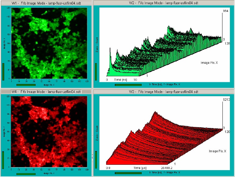
An example of phosphorescence lifetime imaging with the DCS‑120 FLIM system is shown in Fig. 6 and Fig. 7. The images were obtained from particles of an inorganic dye. A BDL‑405 SMC laser was used for excitation; the signals were recorded by the Simple-Tau 152 system of the DCS‑120. Fig. 6 shows images displayed by the SPCM data acquisition software. Lifetime images analysed with the bh SPCImage FLIM analysis software are shown in Fig. 7.

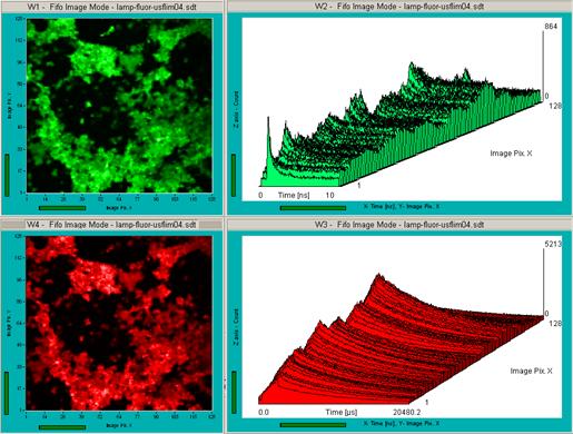
Fig. 6: Fluorescence image (upper left) and phosphorescence image (lower left) recorded simultaneously. ps decay curves and µs decay curves over a horizontal section of the image are shown upper right and a lower right, respectively. Particles of an inorganic luminophore, BDL-405SMC laser, Simple-Tau 152 FLIM system, SPCM data acquisition software.

Fig. 7: Fluorescence lifetime image (left) and phosphorescence lifetime image (right) obtained from the data shown above. Colour scale red to blue 500 ps to 4 ns and 10 to 15 ms, respectively. SPCImage data analysis software.

Zeiss LSM 710 NLO Multiphoton Microscope

To demonstrate simultaneous recording of fluorescence and phosphorescence by two-photon excitation we used a Zeiss LSM 710 NLO multiphoton microscope. An excitation wavelength of 780 nm was used. The luminescence was collected through the non-descanned beam path of the LSM 710. The photons were detected by a Becker & Hickl HPM‑100-40 hybrid detector and recorded by a Becker & Hickl SPC‑150 TCSPC FLIM module [4]. Laser modulation was achieved as shown in Fig. 5.

As a sample we used yeast cells stained with a ruthenium dye. The cells where kept in water in a cell dish, and a small amount of tris(2,2-bipyridyl)dichlororuthenium(II)hexahydrate was added.

Intensity images obtained this way are shown in Fig. 8. Depending on the display parameters set in the TCSPC software different images can be displayed from the same data set recorded. The left image shows the luminescence during the laser-on phases. It contains mainly autofluorescence of the cells, with a small contribution of ruthenium phosphorescence. The image in the middle shows the emission in the laser-off phases. It contains only phosphorescence. Phosphorescence mainly comes from the cell membrane to which the ruthenium dye binds. The image shown right shows the sum of the fluorescence and phosphorescence intensity.

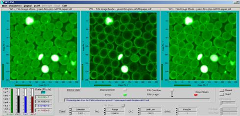
Fig. 8: Intensity images of yeast cells stained with a ruthenium dye. Images from left to right: Fluorescence, phosphorescence, total emission. LSM 710 NLO, two-photon excitation at 780 nm, non-descanned detection, HPM-100-40 hybrid detector, SPC-150 TCSPC FLIM module.

Lifetime images obtained from the same data set are shown in Fig. 9. The fluorescence lifetime image is shown on the left, the phosphorescence lifetime image on the right. Fig. 10 shows decay curves for a selected spot in the images. The blue dots are the photon numbers in the subsequent time channels, the red curve is a fit with a double-exponential decay model, and the green curve is the effective instrument response function (IRF). Please note that the IRF of the fluorescence decay is the laser pulse convoluted with the detector response, whereas the IRF of the phosphorescence decay is the waveform of the laser modulation.

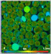
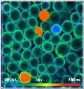
Fig. 9: Fluorescence lifetime image (left) and phosphorescence lifetime image (right) of yeast cells stained with tris(2,2-bipyridyl)dichlororuthenium(II)hexahydrate. Amplitude-weighted mean lifetime of double exponential fit to decay data. Same data set as in Fig. 8, data analysis by Becker & Hickl SPCImage.

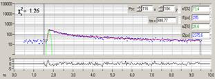
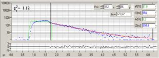
Fig. 10: Decay curves in selected spot of Fig. 9. Left: Fluorescence. Right: Phosphorescence. Blue dots photon numbers in the time channels, red curve fit with double-exponential decay model, green curve effective instrument response function. Inserts: Amplitude-weighted lifetime and double-exponential decay parameters. Decay parameters in ps for fluorescence and in ns for phosphorescence.

Summary

The technique described above simultaneously records fluorescence and phosphorescence lifetime images in confocal and multiphoton laser scanning systems. It eliminates the requirement of using a pulse picker for reduction of the pulse repetition rate, and avoids excessively high pulse power at low excitation rate. The technique can directly be used in the bh DCS‑120 confocal scanning FLIM system. It can easily be implemented in other laser scanning microscopes if these give access to their internal beam blanking control.

Potential applications are oxygen concentration measurements with simultaneous monitoring of cell metabolism via autofluorescence signals, identification of nanoparticles of sunscreens and cosmetical products in the skin, and observation of possible migration of these particles into deep skin layers or inner organs.